Approximately Optimal Approximate Reinforcement Learning

Don't jump to the greedy policy; blend toward it just enough that each round is a guaranteed improvement, and you reach a near-optimal policy in a number of rounds that depends on how good your value estimates are, never on how big the world is.

Read at your level

Start where you're comfortable and climb as far as you like.

• For a 5-year-old
• For a high schooler
• For a college student
• For an industry pro
• For a PhD candidate
• For a peer researcher

Executive summary

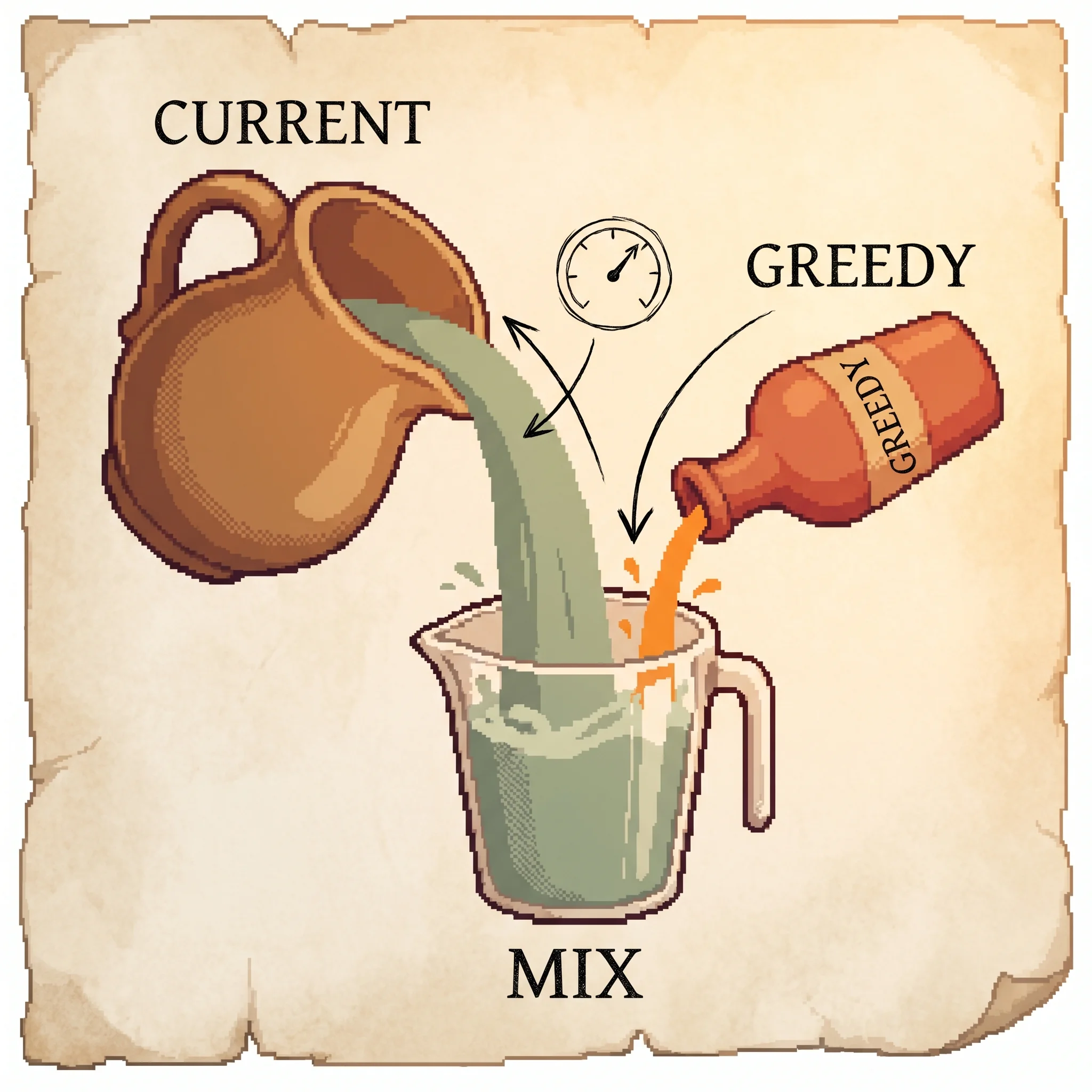
The textbook way to improve a policy is to estimate the value of each move and then switch to always taking the best-looking one. With perfect values that works. With the approximate values you get from any real function approximator it can backfire, because switching changes which situations you face, and the gains you measured under the old behavior don't survive the new one. Kakade and Langford fix this with one careful idea. Instead of replacing the old policy with the greedy one, blend them, mostly the old policy with a small fraction of the greedy move mixed in. They prove the right blend raises performance every single round, and that the algorithm stops at a near-optimal policy after a number of rounds set by how good your value estimates are, not by how many states the world has. The second idea is where you practice from. Optimizing reward measured from the true start ignores states you rarely reach, so the climb stalls there. Restart from a spread of states instead and those rarely-reached corners start to count. The cost is that the guarantee is local and the final gap to optimal grows with a mismatch between where you practiced and where the best policy actually goes. This is the paper that put a trust region under reinforcement learning, and TRPO and PPO are its direct descendants.

Try it

Load Greedy overcommits and press play. The policy curve lurches and drops round after round, because each round jumps all the way to a greedy policy built from noisy value estimates and the ground shifts under it. Switch the update to conservative while it runs and watch the curve stop falling and start climbing. Then load Wrong restart distribution. The mismatch reads infinity and the climb under the true objective stalls below the ceiling. Switch the restart to uniform mid-run and watch the far cells fill with color and the curve resume.

For a 5-year-old

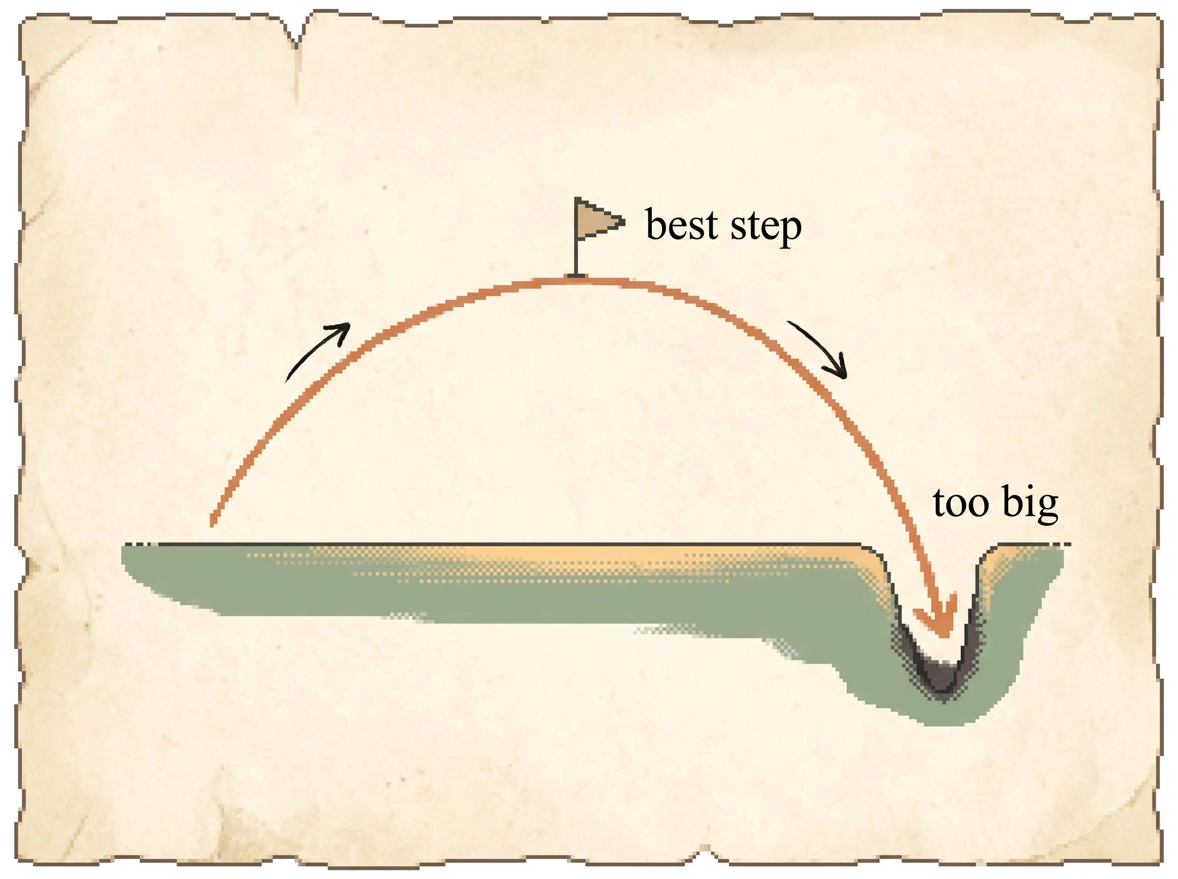
Imagine you're climbing a big hill, but there's fog, so you can only see a little bit around you. You want to get as high as you can.

One way is to look at the foggy shape ahead, guess where the top is, and take a giant leap toward it. The problem is the fog tricks you. Sometimes you leap and land way down low, even lower than where you started. Oops.

A safer way is to take one small careful step uphill. A small step can't trick you. You always end up a little higher than before. Take enough small steps and you climb the whole hill without ever sliding back down.

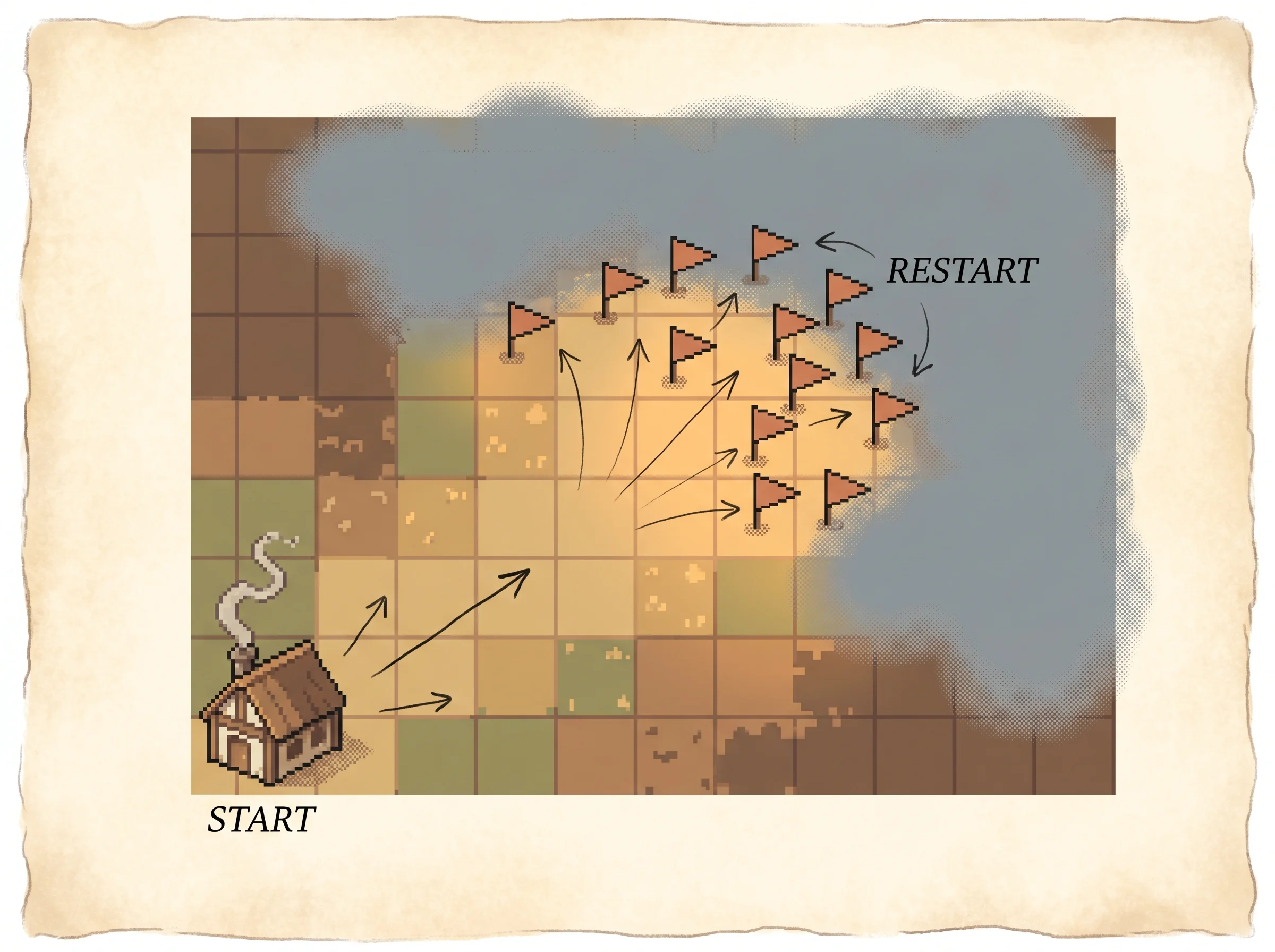
There's one more trick. If you only ever start your climb from your front door, you never learn the far side of the hill, because you almost never walk that far. So you sprinkle little flags all over the hill and practice starting from each one. Now you learn every part, not just the bit near home.

For a high schooler

Think about getting good at a video game. One approach is to rate every situation in your head, "this spot is worth 8, that one's worth 3," and always move toward the higher number. The catch is your ratings are guesses, and they're a little wrong. When you flip to "always chase the highest rating," a tiny mistake in a guess can send you charging the wrong way, and worse, charging that way changes which situations you even run into next. You measured that the move was good while playing your old style. Once you commit to it full-time, you're somewhere new and the measurement doesn't hold.

So don't flip all the way. Keep your current habits and shift them a little toward the better move. Maybe you used to go right here 4 times out of 10, and the better move looks like going right, so you bump it to 5 out of 10. Small shift, small change in where you end up, no nasty surprise. Do that again and again and you steadily get better.

How small a shift? There's a sweet spot. Too tiny and you barely improve. Too big and you're back to the risky full flip. The paper works out exactly how big the shift can be while still being a sure thing.

The last piece is practice variety. If you always start a round from the opening screen, you get tons of practice on early situations and almost none on the rare late ones. So you'd never fix your late-game habits, because they barely affect a score measured from the start. The fix is to start practice rounds from all over the game, not just the beginning. Then every situation counts and you improve everywhere.

For a college student

The setting is a Markov decision process. The agent is in a state s, picks an action a from a policy pi(a; s), lands in a new state, and collects reward. Write V_pi(s) for the expected discounted reward from state s under pi, write Q_pi(s, a) for the value of taking a then following pi, and write the advantage as

A_pi(s, a) = Q_pi(s, a) - V_pi(s)

The advantage is how much better action a is than the policy's own average behavior at s. Positive means "do this more."

Standard policy iteration computes Q_pi, then jumps to the deterministic greedy policy pi'(s) = argmax_a Q_pi(s, a), and repeats. With exact values that improves every step. The trouble is you never have exact values. With an approximate value function carrying error epsilon, the greedy policy is only guaranteed not to get worse by more than 2 gamma epsilon / (1 - gamma). It can drop. There's no guaranteed improvement and no clean quantity to watch.

The conservative fix is to mix instead of replace. Pick a fraction alpha between 0 and 1 and set

pi_new(a; s) = (1 - alpha) pi(a; s) + alpha pi'(a; s)

Now ask how much you'd gain. Define the policy advantage of the greedy policy pi' as the average advantage of its moves, measured over the states your current policy actually visits,

A = E over s ~ d_pi[ A_pi(s, pi'(s)) ]

where d_pi is the discounted distribution of states you visit. Theorem 4.1 then bounds the change in performance:

eta(pi_new) - eta(pi)  >=  (alpha / (1 - gamma)) * ( A - 2 alpha gamma eps / (1 - gamma) )

Read the two terms. The first, alpha A / (1 - gamma), is the gain you'd expect, growing with the step. The second is a penalty growing with alpha squared, because the bigger your step the more the visited states drift away from the d_pi you measured under. The whole thing is an upside-down parabola in alpha.

Maximize that parabola over alpha and you get a guaranteed improvement of A^2 / (8 R) per round, where R is the largest reward (Corollary 4.2). As long as the policy advantage A is positive, the right small step strictly improves performance. That's the whole game. You never take a step you can't prove helps. When A finally drops near zero, no improving direction is left and you stop.

One worked intuition for the penalty. Set alpha = 1 and you've replaced the policy entirely, the second term explodes, and the guarantee goes negative. That's the textbook greedy jump, and the math is telling you it might drop you downhill. Keep alpha small and the guarantee stays positive. The simulation above plots this parabola live. Load the conservative climb, step once, and read the guaranteed gain peak at the safe step and dive negative well before alpha reaches 1.

The last ingredient is where the expectation d_pi starts. If it starts only from the true start state, states far from the start get almost no weight, so improving the policy there barely moves the measured performance and the climb stalls. So you optimize a version that starts from a spread-out restart distribution instead, which weights the whole space more evenly. You improve everywhere, then pay a separate, bounded price for the gap between where you practiced and where the best policy actually spends its time.

For an industry pro

The problem this solves is the one that makes approximate dynamic programming scary to deploy. You learn a value function, you act greedily on it, and because the value function is approximate, the policy can lurch and even degrade from one iteration to the next. There's no monotonic improvement and no principled stopping point. You're flying blind on whether the last update helped.

Conservative policy iteration gives you three guarantees that a deployment cares about. Every update improves a fixed performance metric, so you never ship a regression. The algorithm terminates in at most 72 R^2 / epsilon^2 calls to your value-function-based policy chooser, and that bound does not depend on the size of the state space, only on the reward scale R and the quality epsilon of your chooser. And it returns a policy provably near the chooser's break point. You buy all of this with a single change to the update, blending the new policy in with a small weight instead of swapping it.

Two operational costs are worth stating plainly. First, the guarantee is local, like a gradient method, not global. Second, the metric you're guaranteed to improve is reward measured from a restart distribution you choose, not necessarily reward from your true deployment start state. The gap between them is governed by a mismatch term, how much the best policy's state visitation overshoots the distribution you trained from. Train from a spread of states that covers where good policies go and the gap stays small. Train only from the start state and the bound on that gap blows up.

If you've shipped modern policy optimization you already use the descendants of this paper. The "blend toward the greedy policy by a controlled amount" idea became "constrain how far the new policy can move from the old one," which is the trust region in TRPO and the clipped objective in PPO. The penalty term here, the cost of the visited-state distribution drifting under a big step, is exactly what those methods bound with a KL or total-variation constraint. When you tune PPO's clip range you are choosing this alpha.

For a PhD candidate

The contribution is a policy-improvement scheme with a monotonic guarantee under function approximation, plus a complexity bound free of the state-space size. Three pieces carry it.

First, the conservative update pi_new = (1 - alpha) pi + alpha pi' and its improvement bound (Theorem 4.1). The change in eta_mu decomposes into a first-order term proportional to the policy advantage A and an O(alpha^2) penalty whose constant is the largest per-state expected advantage epsilon = max_s |E_{a ~ pi'} A_pi(s, a)|. The penalty captures the second-order cost of the state distribution d_{pi,mu} shifting away from the one the advantage was averaged under. Optimizing alpha gives eta_mu(pi_new) - eta_mu(pi) >= A^2 / (8 R) (Corollary 4.2). The crucial move is measuring the advantage of pi' under the current policy's visitation d_{pi,mu}, which is observable, rather than under pi_new's visitation, which is not.

Second, the algorithm and its termination (Theorem 4.4). Assume an epsilon-good greedy policy chooser G_eps(pi, mu) returning a pi' whose policy advantage is within epsilon of the best achievable. Estimate A from rollouts under the mu-restart distribution via importance sampling and Hoeffding bounds, take the conservative step, and stop when the estimated advantage drops below the chooser's noise floor. With probability at least 1 - delta this improves eta_mu every update, halts in at most 72 R^2 / epsilon^2 calls to G_eps, and returns a policy with OPT(A_{pi,mu}) < 2 epsilon. The bound's independence from |S| is the headline.

Third, the restart distribution and the mismatch. The reason you optimize eta_mu = E_{s ~ mu}[V_pi(s)] rather than the true eta_D is that eta_D is insensitive to improvement at states D rarely visits, so gradient and greedy methods both stall on plateaus there. The cost is Corollary 4.5,

eta_D(pi*) - eta_D(pi)  <=  (epsilon / (1 - gamma)) * || d_{pi*, D} / d_{pi, mu} ||_inf
                        <=  (epsilon / (1 - gamma)^2) * || d_{pi*, D} / mu ||_inf

The mismatch coefficient || d_{pi*, D} / mu ||_inf is how badly mu under-covers the optimal policy's discounted state distribution. A uniform mu keeps it finite; a mu concentrated on the start leaves it unbounded, which is the simulation's start-only preset reading infinity. The methodological tell is the assumption set, an epsilon-good chooser supplied as a black box and a restart distribution that obviates explicit exploration, both chosen as the minimal machinery that makes the proof go through.

The threats to validity are clearly seen. The chooser's epsilon is assumed, not constructed, and folding it down to an l_1 regression error on the advantages (Section 7.1) is sketched, not proved. Convergence is to a local optimum. And the whole story is built on the restart assumption, which is weaker than a generative model but stronger than single-trajectory experience, so it doesn't apply where you truly can't reset.

For a peer researcher

The delta over greedy approximate dynamic programming is the monotonic guarantee, and the delta over policy gradient is the state-space-free iteration count. Approximate value iteration buys you only the non-degradation bound V_{pi'} >= V_pi - 2 gamma epsilon / (1 - gamma), which permits oscillation and gives no stopping rule. Policy gradient guarantees per-step improvement but, as the same authors' companion analysis and the policy gradient theorem paper make precise, the gradient direction is expensive to estimate exactly when exploration is poor, and the average-reward objective is flat at exactly the unlikely states you most need to fix. Conservative policy iteration takes the policy-improvement framing, replaces the unsafe full greedy step with the largest provably-improving mixture step, and bounds the number of such steps by 72 R^2 / epsilon^2, independent of |S|. That last fact is what makes it "approximately optimal" in a sense that survives large state spaces.

Two pieces became load-bearing for the next two decades. The performance difference lemma (Lemma 6.1), eta_mu(pi~) - eta_mu(pi) = (1 / (1 - gamma)) E_{s ~ d_{pi~, mu}} E_{a ~ pi~}[A_pi(s, a)], is the exact identity that the conservative bound approximates by swapping d_{pi~} for the observable d_pi, and it is the same identity Schulman et al later turn into TRPO's surrogate with a total-variation penalty controlling the swap. The mixture step is the literal ancestor of the trust region, and PPO's clip is the same alpha budget enforced more cheaply. The mismatch coefficient || d_{pi*, D} / mu ||_inf recurs verbatim across the approximate-policy-iteration and policy-search literature as the distribution-mismatch term that gates every sample-complexity result that followed.

What would change my read is the chooser abstraction. The whole apparatus is conditioned on an epsilon-good G_eps, and the reduction to a weighted l_1 regression on advantages is asserted with the harder direction, when does a regressor actually attain that, left open. The estimator's O(n_a^2 R^2 / Delta^2) trajectory cost via Hoeffding is honest but loose, and the importance-sampling step inherits the variance problems the paper criticizes in pure policy gradient, just relocated. None of that dents the core. The conservative step and the performance difference lemma are the two ideas, and essentially every monotonic-improvement policy method since is one or both of them with a different penalty bolted on.

How it works

The problem and why prior approaches failed. Realistic reinforcement learning forces function approximation, because you can't store a number for every state. The dominant approach approximated a value function and read a greedy policy off it. Two failures follow. With value error epsilon, the greedy policy carries only the non-degradation guarantee V_{pi'}(s) >= V_pi(s) - 2 gamma epsilon / (1 - gamma), so it can decline and there's no measure to check improvement against. Policy gradient avoids the discontinuity but stalls on exploration. The paper's two examples are concrete. A chain MDP where reaching the goal under random exploration takes time 3(2^n - n - 1), about 10^15 steps at n = 50, so any on-policy method runs that long before improving. And a two-state MDP where the average-reward landscape has a plateau lasting roughly 10^7 steps because one state's visitation probability sinks to 10^-7, so the gradient there is nearly zero exactly where learning is needed.

The key idea. Improve the policy by mixing toward a better one rather than replacing it.

pi_new(a; s) = (1 - alpha) pi(a; s) + alpha pi'(a; s)

Because pi_new is close to pi for small alpha, the state distribution moves only a little, which is the smoothness the full greedy jump throws away.

The improvement bound (Theorem 4.1). With A the policy advantage of pi' measured under the current visitation d_{pi,mu}, and eps the largest per-state expected advantage,

eta_mu(pi_new) - eta_mu(pi)  >=  (alpha / (1 - gamma)) ( A - 2 alpha gamma eps / (1 - gamma) )

The first term is the gain, the second is the penalty for the state distribution drifting under a larger step. Maximizing over alpha gives a guaranteed gain of A^2 / (8 R) per round (Corollary 4.2). Whenever A > 0, the safe step strictly improves performance.

The algorithm. Conservative policy iteration loops the bound:

loop:
  pi'  <- approximate greedy chooser G_eps(pi, mu)     # usually picks high-Q actions
  A    <- estimate policy advantage of pi' under d_{pi,mu}
  if A < epsilon:  stop and return pi                   # the break point
  alpha <- the step that maximizes the Theorem 4.1 bound
  pi   <- (1 - alpha) pi + alpha pi'

Theorem 4.4 proves that with probability 1 - delta this improves eta_mu every round, stops in at most 72 R^2 / epsilon^2 calls to the chooser, and returns a policy with OPT(A_{pi,mu}) < 2 epsilon. The round count has no |S| in it.

The restart distribution and the mismatch. The metric the loop improves is eta_mu = E_{s ~ mu}[V_pi(s)], reward from a restart distribution mu of your choosing, not the true eta_D from the start state. You do this because eta_D is flat at states D rarely reaches, so improvement there is invisible and the climb stalls. The price is a bounded gap (Corollary 4.5),

eta_D(pi*) - eta_D(pi)  <=  (epsilon / (1 - gamma)^2) * || d_{pi*, D} / mu ||_inf

The mismatch || d_{pi*, D} / mu ||_inf measures how far the best policy's state visitation overshoots mu. Spread mu across the state space and it stays small. Concentrate mu on the start and it can be unbounded, which is why the simulation's start-only restart reads an infinite mismatch and stalls under eta_D while the uniform restart keeps the mismatch near 4 and climbs.

Results. This is a theory paper, so the results are the theorems. Conservative policy iteration is the first policy-improvement algorithm to combine monotonic improvement under approximation with a termination bound independent of the state-space size, and the first to make the restart distribution and its mismatch coefficient explicit. The simulation is the check you can run. The conservative update never drops eta_mu and stops near optimal, the greedy update lurches and degrades, and a start-only restart stalls below optimal under the true objective with an infinite mismatch.

Limitations and open questions. The improvement and termination are local and depend on an epsilon-good greedy chooser that's assumed rather than built, with the reduction to a weighted advantage-regression problem only sketched. The advantage estimate uses importance sampling under mu, which carries variance the bound treats loosely. And the restart assumption, weaker than a full model but stronger than a single trajectory, rules out settings where you genuinely can't reset.

My assessment

This is one of the small number of reinforcement learning papers whose central trick the whole field still runs on, and it earns that with a single honest observation. Switching to the greedy policy is a leap whose landing you can't see, because acting differently changes where you end up, and the value you measured was measured somewhere else. The cure is to take a step you can prove is uphill, which means a small step toward the greedy policy, sized so the gain beats the penalty for the ground shifting under you. Out of that one idea fall the monotonic guarantee, the stopping rule, and a round count that doesn't care how big the world is.

The piece that aged into a foundation is the performance difference lemma. Writing the exact change in performance as the new policy's advantage under its own visitation is the identity that TRPO turns into a surrogate objective and a trust region, and that PPO approximates with a clip. The conservative mixture is the first trust region, written before anyone called it that. The mismatch coefficient is the other lasting export, the term that shows up in nearly every later analysis of why exploration and the choice of training distribution govern how close to optimal you can get.

The honest weaknesses are the ones the next twenty years went to work on. The epsilon-good chooser is a black box, so the paper proves what happens given good value approximation without proving you can get it, and the reduction to a regression problem is a sketch. The estimator relocates the variance of policy gradient rather than removing it. And everything is local and rests on the restart assumption. But none of that is a flaw in the argument so much as an accurate map of the open problems, and the core, take the provably-uphill step and practice from where the good policies go, is as right now as it was then.