Policy Gradient Methods for Reinforcement Learning with Function Approximation

Instead of memorizing the worth of every situation and acting greedily, tune the policy's dials directly along the gradient of expected reward, a gradient you can estimate from experience that never depends on how your tuning shifts which situations you face, and which a value critic shaped to match the policy reproduces with zero bias.

Read at your level

Start where you're comfortable and climb as far as you like.

• For a 5-year-old
• For a high schooler
• For a college student
• For an industry pro
• For a PhD candidate
• For a peer researcher

Executive summary

For a decade the standard way to use a neural network in reinforcement learning was to make it estimate the value of each situation, then act by grabbing the highest-valued move. That approach has a crack in it. A tiny change in an estimated value can flip which move looks best, so the behavior jerks around, and nobody could prove the whole loop converges when the value estimate is approximate. Sutton, McAllester, Singh and Mansour take the other road. They let the network be the policy itself, a knob per situation that sets how likely each move is, and they push those knobs along the gradient of expected reward. Their Theorem 1 writes that gradient in a clean form, an average over the situations you visit of how much you'd nudge each move's probability times how good that move is, and the surprising part is what's missing. There's no term for how tuning the knobs changes which situations come up, so you can estimate the gradient from ordinary experience without a model of the world. Their Theorem 2 is the payoff. Swap the true value for a learned critic and the gradient usually goes wrong, but if the critic is built from the policy's own features, it reproduces the exact gradient with zero bias. From those two results they prove, for the first time, that a policy-iteration loop with general function approximation converges to a locally optimal policy. The cost is that local is all you get, and the estimate is still noisy enough that the critic is what makes it practical. That gradient is the foundation every modern policy method stands on.

Try it

Load An incompatible critic biases it and press play. The alignment light sits below 1.00, the return curve flatlines, and the policy arrows never sharpen toward the goal, because this critic lumps left with right and up with down and can't tell the policy which way to lean. Now switch the critic to compatible while it runs and watch the light snap to 1.00 and the arrows start flowing toward the corner. Then load Follow the true gradient and Swap in a compatible critic back to back and step them together. They move identically, which is Theorem 2 on screen. Finally load Sampled returns (REINFORCE), turn the value baseline off, and watch the light jitter wildly as the variance explodes, then turn it back on to steady the climb.

For a 5-year-old

Imagine a little robot in a maze, trying to reach a shiny star. At every spot the robot has a board of knobs, one for each way it could go. A knob turned up high means "I'll probably go this way." A knob turned low means "probably not."

The robot tries moves and remembers how they went. When a move turns out better than its usual luck at that spot, it reaches over and turns that knob up a little. When a move turns out worse, it turns the knob down. Turn the good knobs up, the bad knobs down, over and over, and the robot drifts toward the star.

Here's the nice part. The robot doesn't have to figure out how turning a knob changes which rooms it ends up in later. That sounds like it should matter, but it quietly cancels out, so the robot can just watch how its moves do and turn knobs. Nothing fancy.

And it has a helper. A little meter can look at a move and say "that one's good, turn it up." A meter built the right way, out of the same knobs the robot uses, always gives advice that's exactly right. A meter built the wrong way will point the robot the wrong way, and it gets lost.

For a high schooler

Think about learning a video game. One way is to rate every situation in your head, "this spot is worth 8, that one's worth 3," and always walk toward the higher number. The other way is to just adjust your habits, "I press jump a little more often right here," and let your reactions get better. This paper is about why the second way is easier to make work.

Rating every situation has a hidden problem. Picture two doors, and you've scored the left one at 5.0 and the right at 5.1. You walk right. Nudge those scores a hair and suddenly the left is 5.1 and the right is 5.0, so you flip and walk left. A tiny change in a number caused a total change in behavior. That jumpiness is why the rating approach is hard to pin down.

The habit approach is smooth instead. Your policy is a set of dials, one per move in each situation, and each dial sets how likely you are to make that move. Turn a dial a little and your behavior changes a little. No flipping.

So how do you know which way to turn each dial? You compare. Keep track of how good a move turned out against how good your moves usually are in that spot. If this move beat your average, turn its dial up. If it fell short, turn it down. That "how much better than average" number has a name, the advantage, and it's the heart of the whole method.

One worked example. Say you're at a fork and you currently go right 4 times out of 10. You try right, and it works out to a value of 8 when your usual at this fork is 6. The advantage is +2, so you bump the dial for "go right" up, maybe to 5 out of 10. Next time you're a touch more likely to do the thing that just beat your average. Had it come in at 4, below your usual 6, you'd have turned that dial down instead.

For a college student

The setting is a Markov decision process. The agent sits in a state s, picks an action a from a policy pi(s, a), lands in a new state, and collects a reward. The policy is parameterized, written pi(s, a, theta), so theta is a vector of knobs and the agent's whole behavior is a smooth function of it. The thing you want to maximize is the performance rho, the expected long-run reward from following the policy. Policy gradient methods just do gradient ascent on it.

theta <- theta + alpha * gradient of rho with respect to theta

The obstacle is that rho depends on theta two ways at once. Changing theta changes which actions you take, and it also changes which states you end up visiting. The second effect looks nasty, because to know how the state-visitation distribution shifts you'd seem to need a model of the environment's dynamics. The paper's first result is that the second effect drops out.

Theorem 1, the policy gradient. Write d(s) for how often you're in state s (a discounted count of visits from the start), Q(s, a) for the value of taking a in s and following the policy after, and V(s) for the average of Q over the policy's own action choices. Then

gradient of rho = sum over s of d(s) * sum over a of (gradient of pi(s, a)) * Q(s, a)

There's no term involving the gradient of d(s). The visitation appears, but never its derivative. That's what makes the gradient estimable from plain experience. If you sample a state by just running the policy, then sum over a of (gradient of pi(s, a)) * Q(s, a) is an unbiased sample of the gradient, and you never had to predict how your own tuning reshapes the states you see.

For a softmax policy, where pi(s, a) comes from exponentiating a preference theta(s, a), the gradient collapses to a rule you can read at a glance:

gradient of rho at theta(s, a) = d(s) * pi(s, a) * A(s, a)
A(s, a) = Q(s, a) - V(s)

Nudge each action's dial by its advantage, scaled by how likely you already are to take it and how often you stand in that state. Advantage above zero pushes the dial up, below zero pushes it down.

You still need Q(s, a), which you don't know. The simplest fix is Williams' REINFORCE. Use the actual return you observed after (s, a) as an unbiased sample of Q, subtract a baseline, and you get an honest gradient with no value function at all. It works, but the returns are noisy, so it learns slowly. The simulation above lets you watch that. The sampled-returns mode climbs in fits and starts, and turning the baseline off makes it lurch much worse.

For an industry pro

The problem this solves is how to train a controller when the thing you optimize isn't differentiable through your model, and you want it to actually converge. The value-function approach that dominated the 1990s, learn Q, act greedily, has two failure modes that bite in production. The optimal policy is often stochastic, and a greedy-on-Q policy can't be stochastic, so it can't represent the best behavior. Worse, an arbitrarily small error in an estimated value can flip the chosen action, which means the policy can lurch discontinuously and the learning loop can fail to settle. Q-learning and Sarsa with function approximation were both shown to be able to diverge.

Policy gradient sidesteps both. You represent the policy directly with its own parameters and move them along the gradient of expected reward. Small parameter changes give small policy changes, so the behavior moves smoothly and the loop has something to converge to. The price is that you converge to a local optimum, not the global one, and the raw gradient estimate is high-variance, so without help it learns slowly.

The help is a critic. Learning a value function and using it in place of the noisy returns is what makes this fast enough to ship, and the paper's Theorem 2 tells you exactly how to do it without poisoning the gradient. Fit a critic, but build it from the policy's own features so it's compatible, and it reproduces the true gradient with zero bias. In today's language that compatible critic is the advantage function, reward-to-go minus a value baseline, and the whole arrangement is an actor-critic. This is the lineage of A2C, A3C, TRPO, and PPO. The RLHF pipeline that aligns large language models is PPO on top of exactly this idea, a policy gradient with a learned value baseline and a trust region to keep each step from lurching too far.

The operating envelope worth remembering. Policy gradient gives you smooth improvement and a convergence guarantee that value methods lack under function approximation, but only to a local optimum, and only on-policy, which means it's sample-hungry. If your action space is small and discrete and a greedy value policy is good enough, a value method may be cheaper. Reach for policy gradient when the optimal policy is stochastic, when the action space is continuous, or when you need the stability that a directly-parameterized, smoothly-updated policy buys you.

For a PhD candidate

The contribution is to express the performance gradient in a form free of the state-distribution derivative, and then to characterize exactly which value-function approximators preserve that gradient. Both formulations are covered, average-reward with rho the reward rate and d the stationary distribution, and start-state with rho the discounted return from s0 and d the discounted state-occupancy. The gradient sum_s d(s) sum_a grad pi(s,a) Q(s,a) holds for both. The average-reward proof leans on stationarity of d, the start-state proof on unrolling V and telescoping. The clean statement supersedes the related expressions from Marbach and Tsitsiklis and from Jaakkola, Singh and Jordan, and it makes Williams' REINFORCE a corollary, since R_t / pi corrects for the oversampling of likely actions and rides the same gradient in expectation.

Theorem 2 is the part that earns the title. Approximate Q with f_w and the gradient is generally biased. But require two things. First, f_w is compatible, meaning grad_w f_w(s,a) = grad_theta log pi(s,a), so the critic's features are the policy's score features. Second, w is at a least-squares optimum under the on-policy weighting d(s) pi(s,a). Then the approximation error is orthogonal to the policy's score features, you can subtract it from the policy gradient for free, and f_w substitutes for Q exactly. For a Gibbs policy linear in features phi_sa, compatibility forces

f_w(s, a) = w . (phi_sa - sum_b pi(s, b) phi_sb)

which is mean-zero over actions in every state. So f_w can't represent V(s) at all, only the relative value of actions. The honest reading, which the authors state, is that f_w approximates the advantage, not the action-value. A state-dependent baseline v(s) can be added back without touching the gradient, since sum_a grad pi(s,a) = 0, and it should be set near V(s) to cut variance. This is the theoretical home of the advantage function and of the baseline trick that earlier work used on faith.

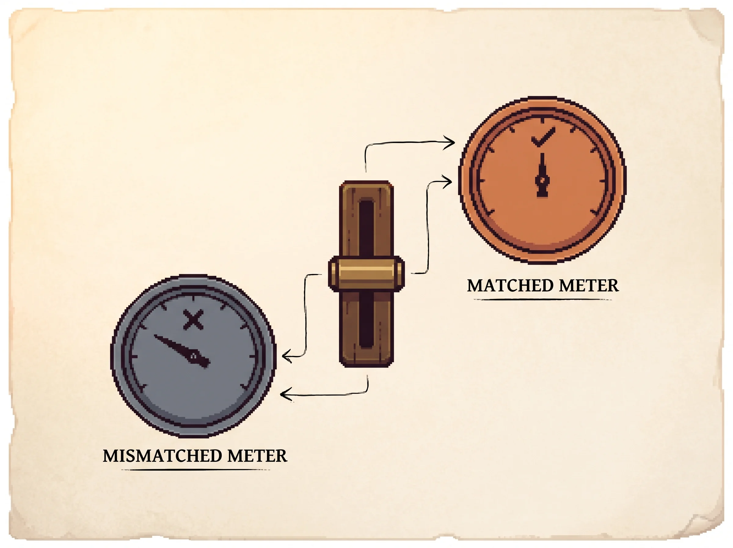
The simulation makes the compatibility condition tangible. The incompatible critic there collapses the four actions into two axis-groups, so it can't distinguish actions the policy distinguishes, its error is no longer orthogonal to the score features, and the gradient it produces is biased. The alignment readout, the cosine against the exactly-computed gradient, holds at 1 for the compatible critic and drops for the incompatible one. That cosine is the inner product at the center of the orthogonality argument, made visible.

Theorem 3 closes the loop. With a policy and a compatible critic that are differentiable with bounded second derivatives, with the critic fit to its least-squares optimum at each iteration, and with Robbins-Monro step sizes, the sequence of policies converges so that the gradient vanishes. It's the first convergence result for policy iteration with general differentiable function approximation, and it stands in deliberate contrast to the divergence results for value-based methods with approximation. The methodological choices read as the minimal set that makes the proof go through, and the open seams are clear, a local optimum rather than global, the assumption that the critic is fully fit before each policy step, and a variance story the theorem doesn't quantify.

For a peer researcher

The delta over Williams is precise. REINFORCE already gives an unbiased gradient from sampled returns, but it can't use a learned value function without, in general, biasing the estimate, which is why it's slow. This paper identifies the exact subspace of value approximations that leave the gradient intact, the ones compatible with the policy parameterization, and proves equality with the gradient rather than the weaker positive-inner-product result of Jaakkola, Singh and Jordan for the tabular-POMDP case. That upgrade from "points roughly uphill" to "is the gradient" is what licenses the convergence proof.

The choices are deliberate and worth contesting on their own terms. Compatibility is stated as a constraint linking the critic's features to the policy's score function, and the footnote concedes that linear-in-the-policy-features may be the only way to satisfy it, which quietly bounds how expressive a bias-free critic can be. The least-squares optimum under d(s) pi(s,a) is the weighting that makes the error orthogonal to the score features, and any other weighting breaks the result, so the on-policy distribution isn't a convenience here, it's load-bearing. Folding an arbitrary v(s) back in is shown to leave the theorems untouched while changing variance, which reframes the baseline as a pure variance instrument and the critic as an advantage estimator, the cleaner mental model that the field adopted.

What would change my read is the variance and the two-timescale gap. Theorem 3 assumes the critic reaches its least-squares optimum before each policy update, which practice replaces with a faster critic timescale, and the convergence and variance behavior of the coupled iteration is exactly what Konda and Tsitsiklis and the later actor-critic literature had to work out. The result is also resolutely local, and Michael Kearns is thanked for insights into what "optimal under function approximation" even means, a hint that the global picture was understood to be unsettled. None of that diminishes the core. Every on-policy policy gradient method in use descends from these two theorems, the gradient form and the compatible critic, and the advantage function and GAE are direct readings of the baseline-and-advantage argument tucked into Section 3.

How it works

The problem and why prior approaches failed. Function approximation is unavoidable in any real reinforcement learning problem, because you can't store a separate number for every state. For a decade the standard move was to approximate a value function and read a policy off it by acting greedily. Two things go wrong. The optimal policy is often stochastic, and a greedy policy can't be, so the representable policies exclude the best one. And the policy is a discontinuous function of the values, so an arbitrarily small change in an estimated value can flip an action in or out, which both breaks the smoothness any convergence argument wants and was shown to let Q-learning and Sarsa diverge under approximation.

The key idea. Represent the policy with its own function approximator, separate from any value function, and update its parameters along the gradient of expected reward.

theta <- theta + alpha * (gradient of rho with respect to theta)

Because the policy is a smooth function of theta, a small step changes the behavior and the state-visitation only a little, which is exactly the smoothness the value approach lacked.

Theorem 1, the gradient in an estimable form. The performance gradient is an average over visited states of how you'd nudge each action's probability, weighted by that action's value.

gradient of rho = sum over s of d(s) * sum over a of (gradient of pi(s, a)) * Q(s, a)

The crucial absence is a term for the gradient of d(s). Tuning the policy shifts which states you visit, and you'd expect to pay for that in the gradient, but it cancels, in the average-reward case because d is stationary and in the start-state case because the unrolled value terms telescope. So you can sample states by just running the policy and form an unbiased gradient estimate with no model of the dynamics. For a softmax policy this is the per-knob rule the simulation applies, d(s) * pi(s, a) * A(s, a), where A = Q - V is the advantage.

REINFORCE as the first estimator. You still need Q. Use the observed return after each action as an unbiased sample of it, subtract a baseline, and you have Williams' REINFORCE, a policy gradient with no critic. It's unbiased but high-variance, which is why it learns slowly, and it's the noisy mode you can switch to in the simulation.

Theorem 2, a critic that doesn't bias the gradient. Replacing Q with a learned f_w generally biases the gradient. It stays exact under two conditions. The critic must be compatible, its features equal to the policy's score grad log pi, and it must sit at a least-squares optimum under the on-policy weighting. Then the critic's error is orthogonal to the policy's features and drops out.

critic features(s, a) = gradient of log pi(s, a)
fit w by weighted least squares to the returns
gradient of rho = sum over s of d(s) * sum over a of (gradient of pi(s, a)) * f_w(s, a)   # exact

For a softmax policy the compatible critic is forced to be mean-zero over actions in each state, so it represents the advantage, not the value. A state-value baseline can be added back for free to cut variance.

Theorem 3, convergence. Alternate two steps, fit the compatible critic to its optimum, then take a gradient step on the policy, with step sizes that shrink but don't vanish too fast. For any MDP with bounded rewards this converges so the gradient goes to zero, a locally optimal policy. It's the first such guarantee for policy iteration with general differentiable function approximation, in pointed contrast to the divergence that value-based approximation can suffer.

Results. This is a theory paper, so the results are the three theorems and their proofs, not benchmark numbers. The contribution is the gradient form free of the state-distribution derivative, the exact characterization of bias-free critics, and the convergence proof. The simulation is the empirical check you can run yourself, the exact and compatible critics hold the alignment at 1 and climb to optimal, the incompatible critic biases the gradient and stalls, and the sampled-returns mode is unbiased but visibly noisy.

Limitations and open questions. Convergence is to a local optimum, not a global one. The proof assumes the critic is fully fit before each policy update, which practice replaces with a faster-learning critic and a coupled two-timescale analysis the paper doesn't carry out. The gradient estimate's variance is real and unquantified here, and is what the critic and later tricks exist to tame. And for common policies the compatible critic is essentially forced to be linear in the policy's features, which caps how expressive a strictly bias-free critic can be.

My assessment

This paper is the hinge the whole field turned on, and it earns that by doing two unglamorous things exactly right. It writes the gradient in the one form that's actually estimable, with no state-distribution derivative, and it says precisely which learned critics you're allowed to plug in without lying to the gradient. Everything downstream is built on those two sentences. The advantage function, actor-critic methods, A3C, TRPO, PPO, and the RLHF loop that tunes today's language models are all the compatible-critic policy gradient with progressively better variance control and step-size discipline bolted on. Strip PPO down to its core and you find Theorem 1 with the Theorem 2 critic.

What the authors got right beyond the math is the framing of the contrast. They diagnosed the exact disease of the value-function approach, that a hair's change in an estimated value flips the policy, and they prescribed the cure, parameterize the policy so it moves smoothly, and then they proved the cure converges where the disease diverges. That's a complete argument, problem to theorem, and it's why the paper reads as inevitable in hindsight.

The honest weaknesses are the ones the field then spent twenty years on. Local optima are all you're promised. The convergence proof assumes a luxury, a fully-fit critic at every step, that real systems can't afford, so the practical algorithm is a two-timescale approximation the theorem doesn't cover. And the variance that makes the bare estimator slow is acknowledged but not bounded. None of that was a flaw in the work so much as a correct map of the next decade. The single move that aged best is the quiet reframing in Section 3, that the compatible critic is really an advantage approximator and a value baseline rides along for free. That one paragraph is the seed of generalized advantage estimation and of the advantage-centric view that every modern implementation takes for granted.