Scaling Laws for Neural Language Models
A language model's error drops along a clean, predictable line as you grow its size, its data, or its compute, and the best way to spend a fixed compute budget is to mostly build a bigger model.
Read at your level
Start where you're comfortable and climb as far as you like.
- For a 5-year-old
- For a high schooler
- For a college student
- For an industry pro
- For a PhD candidate
- For a peer researcher
Executive summary
People used to guess about how to build a better language model. Make it deeper, make it wider, tune the knobs, hope. This paper turned the guessing into arithmetic. The authors trained hundreds of Transformers across a billion-fold range of sizes and found that the test loss falls as a power law in three things: the number of parameters N, the size of the dataset D, and the compute C spent training. Plot the loss against any one of them on log-log axes and you get a straight line, holding for more than seven orders of magnitude. The shape of the network barely matters. Because the laws are so clean, you can predict the loss before you train, and you can solve for the best way to split a fixed compute budget. The answer surprised the field. Spend most of new compute on a much bigger model, feed it only a little more data, and stop training well before it converges. The catch is that these are empirical fits on one dataset, and the lines must bend somewhere, since natural language has a floor the loss can't drop below.
Try it
Load the Loss vs model size preset and press play. Watch the loss draw itself out as a dead-straight line down six orders of magnitude. Then load Optimal budget split, drag the allocation slider down toward a small model, and watch the realized loss climb above the floor while the overfit reading stays low. Now drag it up past 1 and the overfit reading climbs instead, because the model has outgrown the data its budget can buy.
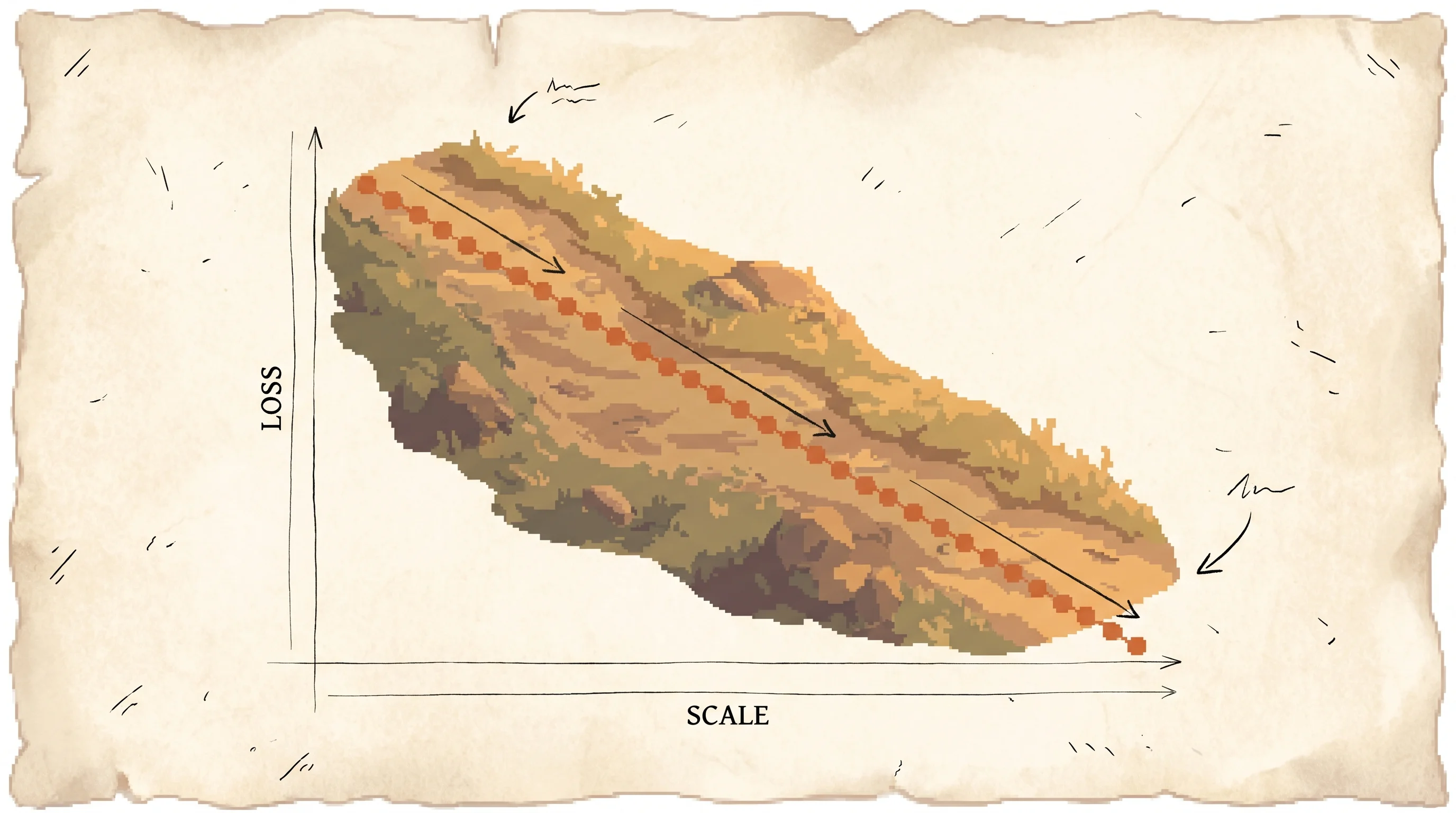
Grow only the model and watch the loss fall along a dead-straight line in log-log. Press play and the curve draws itself out over six orders of magnitude.
Hold data and compute out of the way and grow only the model. The loss tracks a straight power law in N with slope 0.076.
| compute C | 1.0e0 PF-days |
| optimal N* | 1.3e9 |
| your model N | 1.3e9 |
| tokens D | 1.1e10 |
Step, flip the axis, or drag a control to start the log.
The curves come straight from the paper's fitted power laws, L(N) = (Nc / N)^0.076, and the allocator uses the combined L(N, D) fit with the optimal split N* ≈ C^0.73. The numbers are the paper's WebText2 fits, not a fresh training run. The empirical scatter on the points is seeded and deterministic per preset; press “Reshuffle empirical scatter” to see a different noise sample, which illustrates that the power-law trend holds regardless of which noise draw you pick.
For a 5-year-old
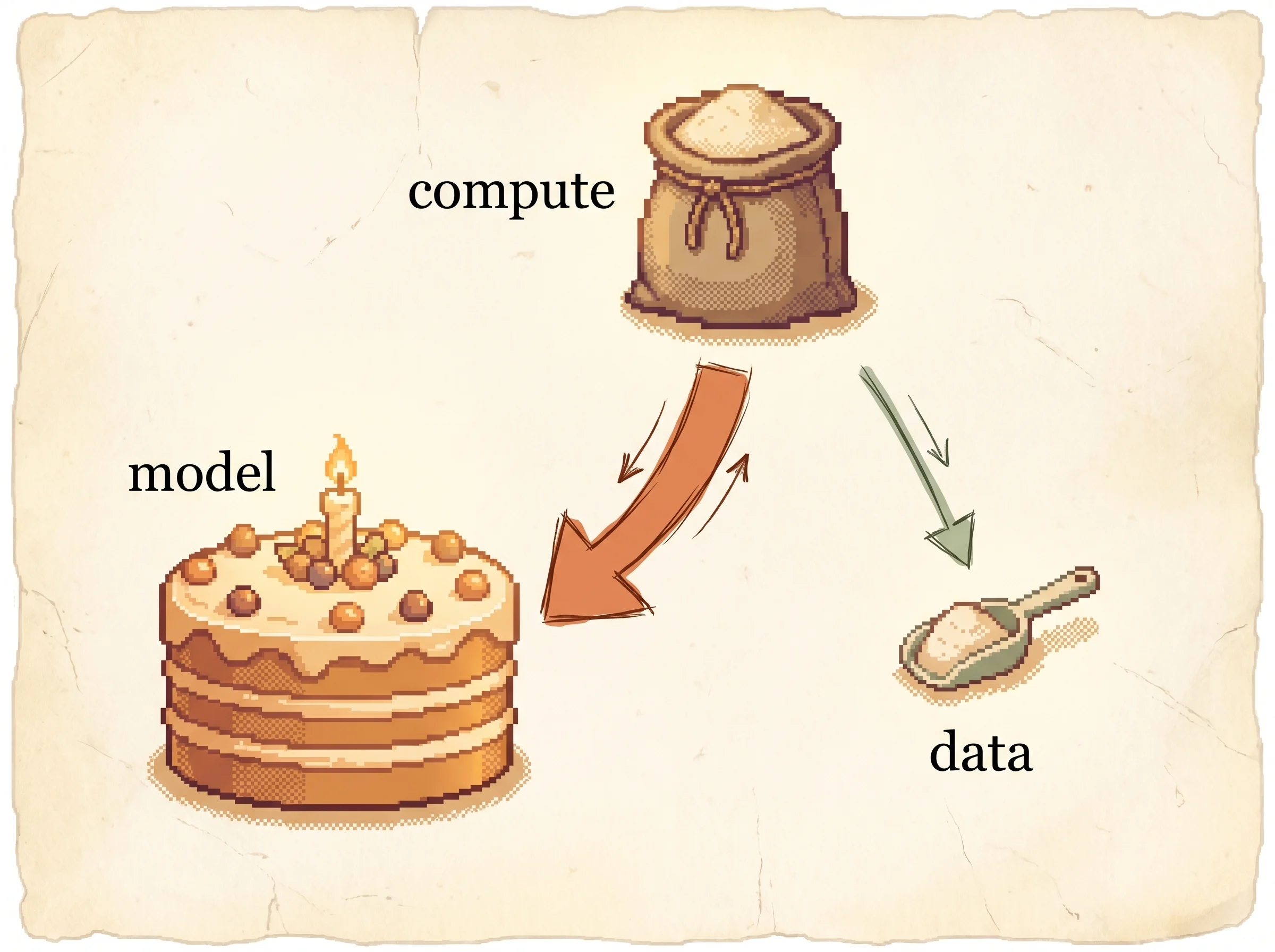
Imagine you're learning to bake a cake, and you want it to taste better and better. Three things can help. A bigger cake pan. More batter. More time in the oven.
Here's the magic. If you make all three a little bigger, the cake gets a little better, every single time, in a way you can count on. Double the size, it gets better by the same amount. Double it again, better by the same amount again. The improvement comes in steady steps, like climbing down a staircase one stair at a time.
Now you have one bag of flour and that's all you get. Where should it go? Into a bigger pan, or into extra batter? The bakers in this story found the answer. Put almost all of it into a bigger pan, and only a tiny bit into extra batter. A big pan with a little batter beats a small pan crammed full.
Cakes don't really have a loss number, and a model isn't baked in an oven. The model is doing math on a giant pile of words, and the loss is just how surprised it is by the next word. But the feeling holds. Make it bigger and it gets better, one steady step at a time.
For a high schooler
You've seen graphs where a line goes up or down steadily. A power law is a special kind. It looks curved on a normal graph, but if you stretch both axes so each step counts times-ten instead of plus-one, the curve straightens into a perfect line. That stretched graph is called log-log, and almost every result in this paper lives on one.
Here's the one idea for this section. The authors measured a model's loss, which is how badly it predicts the next word. Lower is better. They changed three things one at a time. The model's size (how many numbers it has to learn, called parameters). The amount of training text. The total computing work. Each time, the loss dropped along a straight log-log line. A straight line means the rule never changes. The hundredth doubling helps as much as the first.
Try a worked example with the paper's numbers. The loss from model size follows L = (Nc / N) raised to the 0.076 power, where Nc is a fixed constant. Make the model 10 times bigger and the loss multiplies by 10 to the negative 0.076, which is about 0.84. So every 10x in size cuts the loss to roughly 84 percent of what it was. Do it again, another 84 percent. Small steps, but they never stop and they never shrink.
The payoff is that you can predict the future. Measure a few small models, draw the line, and read off how good a giant one will be before you build it.
For a college student
You should care about this because it is the reason the field started spending tens of millions of dollars on single training runs with confidence instead of hope. If the loss follows a known curve, a compute budget becomes an investment with a forecastable return.
The core result is three power laws, each holding when the other two factors are abundant enough not to bottleneck the run. With N the non-embedding parameter count, D the dataset in tokens, and C the compute in petaflop-days:
L(N) = (Nc / N)^0.076       Nc ≈ 8.8 × 10^13
L(D) = (Dc / D)^0.095       Dc ≈ 5.4 × 10^13
L(C) = (Cc / C)^0.050       Cc ≈ 3.1 × 10^8
Each is a straight line in log-log space with slope equal to the negative exponent. The exponents are small, so progress is slow per decade, but it is dead steady. The simulation draws exactly these lines. Switch the axis between model size, data, and compute and the slope changes but the straightness never does.
The deeper result combines model size and data into one equation, so you can ask what happens when neither is abundant.
L(N, D) = [ (Nc / N)^(αN/αD) + Dc / D ]^αDRead the two terms. The first depends only on N and is the floor you hit with infinite data. The second depends only on D and grows as the dataset shrinks. When D is huge the second term vanishes and you recover L(N). When D is small the second term dominates and the model overfits, learning the training set instead of the language.
The overfitting penalty depends almost entirely on the ratio N^0.74 / D. That single number tells you whether a model is starved for data. The practical rule that falls out is that to grow a model 8x without overfitting, you only need about 5x more data. Data needs grow slower than model size, which is the seed of the headline finding.
Here is one path end to end. Fix a compute budget C. The compute spent is roughly C ≈ 6ND, so once you pick N the dataset D is whatever the budget leaves. The combined law then tells you the loss. Sweep N from small to large and the loss traces a U. Too small a model wastes the budget on data it can't use. Too large a model starves for data and overfits. The bottom of the U is the optimal split, and the paper finds it sits at N* ∝ C^0.73. Most of any extra compute should go to a bigger model.
The limitation is built into the math. A power law with no floor predicts the loss reaches zero, which is impossible because language has irreducible entropy. The lines must bend eventually. The paper is honest that it never saw the bend.
For an industry pro
The problem this solves is budget planning for training. Before this, you sized a model by intuition and found out if it was right after spending the compute. Scaling laws turn that into a forecast. Fit the curve on cheap small runs, then read off the loss a large run will hit, and the model size that minimizes loss for your budget.
What it costs you to use is almost nothing. The inputs are parameter count, token count, and compute, all of which you already track. The fits in the paper are for Transformers on a WebText-style corpus, so treat the exact constants as a starting point and refit on your own data and tokenizer, since those constants have no fundamental meaning and shift with vocabulary.
The expected improvement over the old instinct is large and counterintuitive. The old instinct trained a modest model on as much data as possible, to convergence. This paper says do the opposite. With a fixed budget, train a much bigger model, on relatively little data, and stop early, well short of convergence. Bigger models are more sample-efficient, so they reach a given loss in fewer steps and on fewer tokens. The optimal model size grows about 5x for every 10x of compute, while the data processed grows only about 2x.
The failure mode to plan around is that this paper's split is not the last word. It points toward very large, undertrained models. A later result (the Chinchilla paper) refit the curves with a corrected setup and found data should scale closer to one-for-one with model size, which means this paper undertrains its data. So use the method, but refit the exponents rather than trusting these specific numbers for a frontier run. The operating envelope also has a ceiling nobody has measured, since the laws must break before the loss hits the entropy of language.
For a PhD candidate
The contribution is a precise, multi-decade empirical characterization of how Transformer language-model loss depends on N, D, and C, plus a closed-form L(N, D) and a derivation of the compute-optimal frontier from it. Prior work had found power-law-ish relationships between performance and dataset or model size, but piecemeal and over narrow ranges. The delta here is the simultaneous fit, the cleanliness across seven orders of magnitude, and the demonstration that architecture (depth, width, head count, feed-forward ratio) is nearly irrelevant once you hold non-embedding N fixed.
The methodological choices reward attention. Defining N as non-embedding parameters is what makes the L(N) trend collapse cleanly across depths, since embedding parameters scale with vocabulary and contaminate the count. The L(N, D) functional form is chosen from three stated principles: it must rescale under vocabulary changes, it must reduce to L(N) and L(D) in the right limits, and it must be analytic in 1/D at large D so overfitting admits a 1/D expansion. That last principle is the speculative one, justified by an analogy to dataset signal-to-noise rather than measured. The training-time law L(N, S) introduces Smin, the step count adjusted to the critical batch size from the gradient-noise-scale work, so that runs at different batch sizes become comparable. The compute-optimal exponents then follow analytically, αC_min = 1/(1/αS + 1/αB + 1/αN) ≈ 0.054, and match the empirical fit closely.
The threats to validity worth probing. The fits use a fixed batch size for the basic compute trend, which the authors themselves flag as suboptimal and correct for later with Bcrit, so the raw L(C) and the adjusted L(C_min) differ. The early-stopping and overfitting analyses fix dropout and do not optimize regularization across the sweep, so the overfitting curve may be pessimistic where regularization could help. The smallest-dataset runs (reduced by 1024x) break the fit, hinting at a different regime early in training. And the whole edifice is one corpus, so universality across modalities is conjecture. The open question they pose, where and why the laws bend, became the central question the field chased next.
For a peer researcher
The delta against the scattered prior scaling results is the joint, clean, wide-range fit and the move from observation to prediction. The L(N, D) ansatz plus the Bcrit-adjusted L(N, Smin) lets them derive the compute-efficient frontier rather than just plot it, and the derived and empirical exponents agree, which is the strongest internal check in the paper.
The choices read as deliberate tradeoffs. Non-embedding N over total parameters buys depth-independence at the cost of a count that doesn't match what practitioners report. The 1/D-analytic form for L(N, D) buys a clean overfitting law at the cost of a principle they admit is weak. Fitting at fixed batch size buys simplicity in Section 3 and forces the Bcrit correction in Sections 5 and 6, where the cleaner trends live. The compute-optimal recommendation, N* ∝ C^0.73 with data growing only as C^0.27, is the load-bearing claim, and it is exactly where the most consequential later disagreement landed.
What would change my mind, and partly did. If a corrected experimental setup moved the data exponent materially, the undertrained-giant recommendation would weaken. That is what happened. Chinchilla refit with a properly tuned learning-rate schedule and per-budget early stopping and found N and D should scale together, roughly one-for-one, implying this paper systematically undertrains its data. The scaling-law method survived intact; the specific allocation did not. The honest soft spot the authors named, that power laws with no floor predict impossible zero loss and must bend before some L*, is still open, and their conjecture that the bend marks the entropy of natural language remains a conjecture.
How it works
The problem and why prior approaches failed. Picking a language model meant guessing at architecture and size, then training to find out. Earlier scaling studies existed but covered narrow ranges and didn't combine factors, so they couldn't tell you how to trade model size against data against compute. Without that, a compute budget had no principled allocation.
The key idea. Measure the loss across a billion-fold range of N, D, and C, and discover that each relationship is a power law, clean enough to predict from and to combine. Power laws are straight lines in log-log space, so the rule is the same at every scale.
Methodology. The authors trained decoder-only Transformers on WebText2, from a few hundred to 1.5 billion non-embedding parameters, on datasets from 22 million to 23 billion tokens, varying shape, context length, and batch size. They measured cross-entropy loss on held-out text. Defining N as non-embedding parameters is the move that makes the trends collapse cleanly.
N ≈ 12 · n_layer · d_model^2     (non-embedding parameters)
C ≈ 6 · N · D                    (training compute, PF accounting)
The three single-factor laws hold when the other two don't bottleneck. To handle the case where both N and D are limited, they fit one combined equation.
L(N, D) = [ (Nc / N)^(αN/αD) + Dc / D ]^αDThe overfitting penalty, how much worse finite data makes the loss, depends on the combination N^0.74 / D alone, which is why growing a model 8x needs only about 5x more data to stay safe. Load the Optimal budget split preset in the simulation and drag allocation down to see the realized loss rise above the floor as the model starves.
Results with effect sizes. The loss follows L(N) = (Nc/N)^0.076, L(D) = (Dc/D)^0.095, and L(C_min) = (Cc/C_min)^0.050, each straight over six to eight orders of magnitude. Architecture barely matters: changing the aspect ratio (depth versus width) by 40x moves the loss only a few percent. The compute-optimal model size scales as N* ∝ C^0.73, so a 10x compute increase calls for roughly 5x more parameters and only about 2x more data, with the number of training steps barely growing at all. Larger models hit a target loss in fewer steps and on fewer tokens, so compute-optimal training stops far short of convergence.
Limitations and open questions. The laws are empirical fits on one corpus with fixed regularization, and the smallest-dataset runs already break them. A power law with no floor predicts zero loss, which language forbids, so the trends must bend before some loss L*. The authors estimate that intersection point but can't reach it, and they leave open whether the laws transfer to other modalities and what theory would derive them.
My assessment
The authors got the central method right, and it reshaped how the field spends money. Turning model design into a forecast you can fit on cheap runs and extrapolate is the kind of result that changes behavior, and it did. The finding that architecture is nearly irrelevant next to scale was liberating and largely held up. The cleanliness of the lines over seven orders of magnitude is the rare empirical result that feels almost like a law of nature, and the analogy the authors reach for, thermodynamics relating macroscopic properties without tracking every molecule, is apt.
Where they got it wrong is specific and important. The headline allocation, train a giant model on relatively little data and stop early, came from fits made at a fixed batch size with unoptimized early stopping. Chinchilla redid the experiment with a corrected setup and found data should scale about one-for-one with model size, which means this paper's recommendation systematically undertrained its data and pointed the field toward models bigger and hungrier than they needed to be. That is a real miss, and a costly one, since a lot of compute went into oversized, undertrained models in the years between. But it is a miss within the framework the paper built, not a refutation of it. The method was right; the constants were off. What's next was set by the soft spot the authors named themselves. The lines must bend, and finding where, and what the floor means, is still the open question.