Learning from Delayed Rewards

An agent can learn the best thing to do in every situation with no map of its world, just by edging a table of move-by-move scores toward each reward it bumps into, until the value of a distant goal seeps backward through every step that leads to it.

Read at your level

Start where you're comfortable and climb as far as you like.

• For a 5-year-old
• For a high schooler
• For a college student
• For an industry pro
• For a PhD candidate
• For a peer researcher

Executive summary

The hard part of learning to act is that the payoff comes late. You make a move now, and the reward or the disaster shows up many moves later, so you can't tell which earlier move to thank or blame. The old answer was dynamic programming, which solves this cleanly but needs a full map of the world, every rule for how it moves and what it pays. Chris Watkins' 1989 thesis throws the map away. His agent keeps one number for every move it could make in every situation, a score for "how good is it to do this here," and after each real step it nudges that one number a little toward the reward it just got plus the best score available where it landed. Do this enough, trying every move in every spot, and the scores converge on the truth, and reading off the highest-scoring move in each spot gives an optimal way to act. He proved it converges. The cost is that the agent needs a score for every situation-and-move pair and has to visit them all many times, so the plain version doesn't stretch to huge or continuous worlds without extra machinery. That algorithm is Q-learning, and almost all of modern reinforcement learning grows from it.

Try it

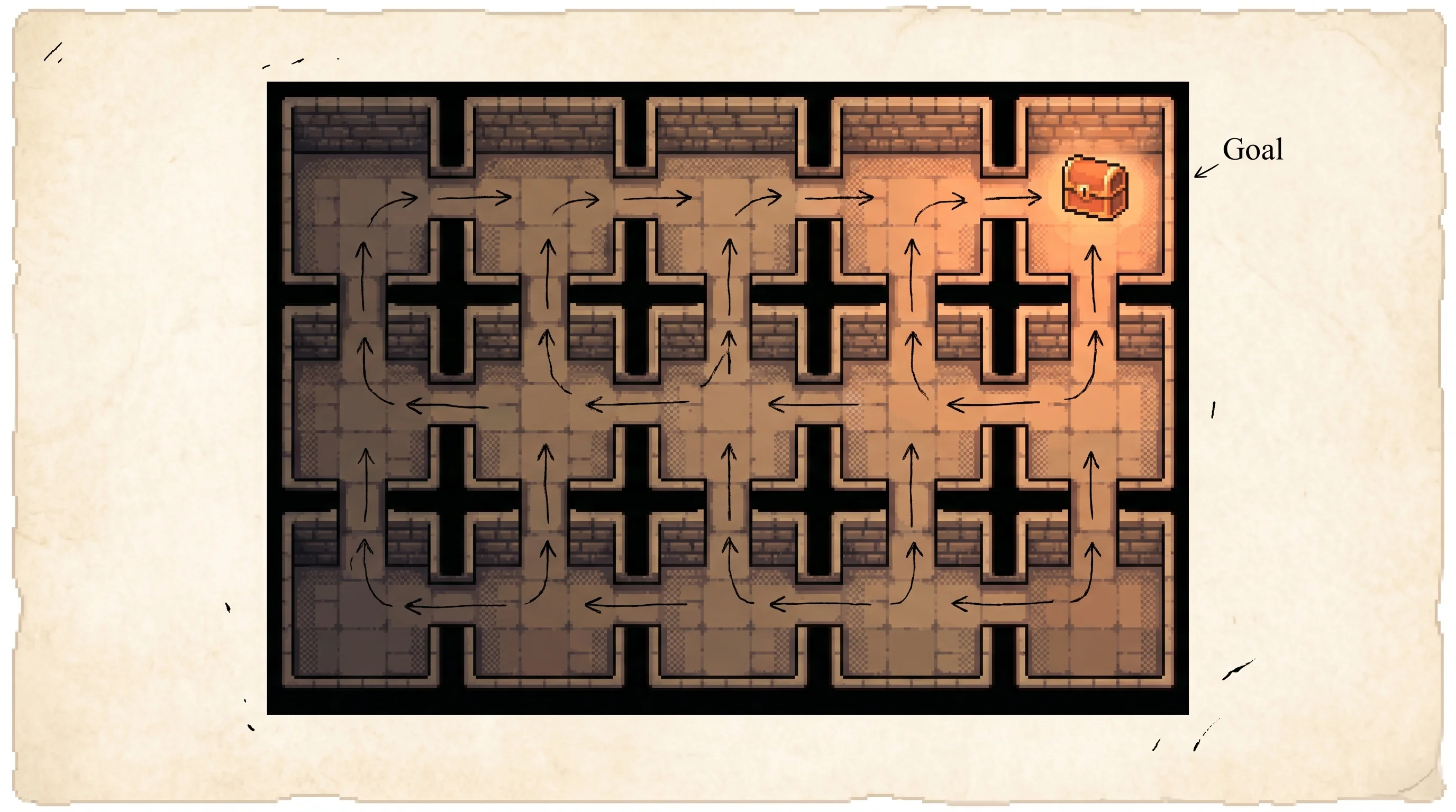
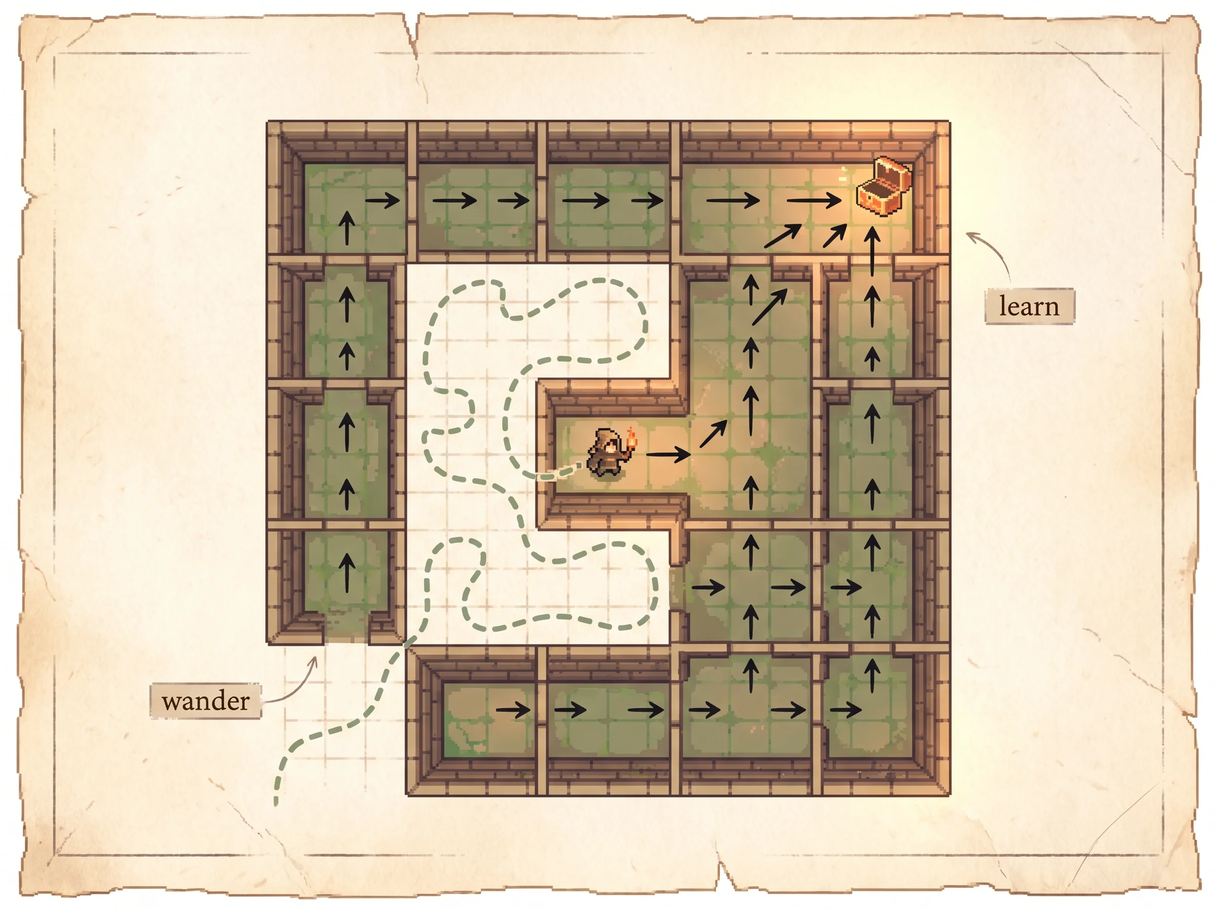
Load Value backs up and press play. The orange glow crawls out from the goal one cell at a time, and the arrows snap into a path that threads the maze. Once it's solved, click a cell on that path to drop a wall across it, and watch the agent bump the new wall, the value drain out of the dead end, and a fresh route fill in. Then load Off-policy: pure random and notice the agent staggers around with no plan at all while the arrows still settle onto the best route. That gap, between how it moves and what it learns, is the whole trick.

For a 5-year-old

For someone brand new to all of this.

Imagine a treasure chest hidden deep in a maze of rooms. You want to find it, but the maze is big and you don't have a map.

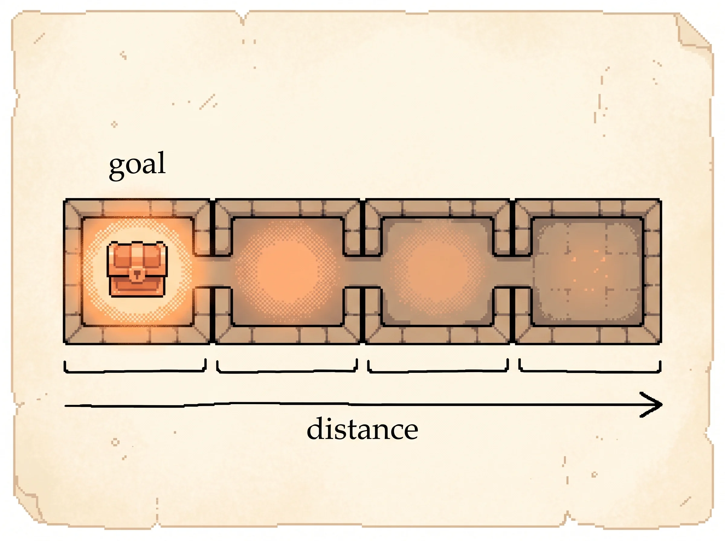
So you wander. You open doors, you walk into walls, you go in circles. Boring. But the moment you bump into the room with the treasure, something nice happens. That room glows. And here's the magic. The glow spreads. The room right next to the treasure starts to glow a little too, because it's one step away from something good. Then the room next to that one glows a little less, and so on, the warm light leaking backward through the maze.

Now you don't need a map. From any room, you just walk toward the brighter room. Follow the glow and it carries you to the treasure every time.

The doors don't really glow, and nobody is holding up a lantern. The glow is a number the maze-walker keeps in its head for every door, a guess at how close that door gets you to the treasure. Every time it takes a step, it fixes up one number a tiny bit. After enough wandering, the numbers are right, and the brightest door is always the way to go.

For a high schooler

If you've seen a bit of algebra and played a video game with a map.

Think about how you learned a level in a game. The first time through you died a lot and had no idea which turn was the good one. After enough tries you just knew, this corridor leads somewhere good, that one is a dead end. Nobody handed you the level's blueprint. You built that sense from playing.

That's the problem this thesis solves. The agent lives in a world of situations, called states, like which room you're in. In each state it can pick from a few actions, like which door to take. Some moves eventually pay off and some don't, and the catch is that the payoff is late. You grab the treasure twenty steps after the turn that mattered, so you can't easily tell which turn to credit. That late payoff is the "delayed reward" in the title, and it's the thing that makes this hard.

Here's the move. For every door in every room, the agent keeps a single number, call it the door's score. The score means "if I take this door and then play well after, how much reward do I expect in the end." Every time the agent actually takes a door, it gets a small reward or cost right then, and it lands in a new room. It looks at the best score among that new room's doors, adds the reward it just got, and slides the door it took a little toward that total.

Picture two rooms. You leave the "now" room through a door, you collect whatever reward sits between them, and you arrive in the "next" room, which already has a glow that says how good it is from there. You feed that glow back to update the score on the door you just used.

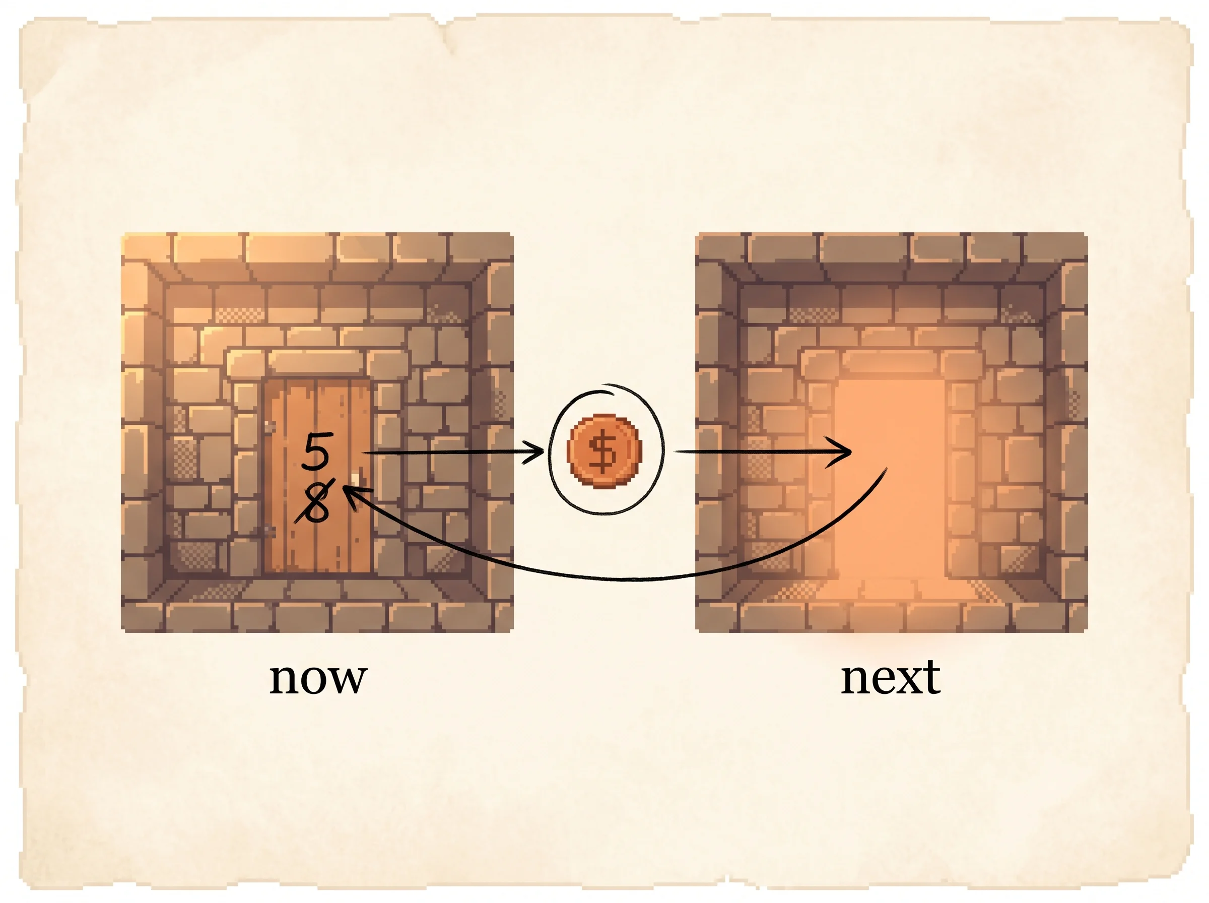
Do that over and over. The room with the treasure pushes its value into its neighbors, they push it into theirs, and the good news flows backward through the whole world one step at a time.

One more knob matters. A reward far away is worth a bit less than the same reward right now, so each step back the glow dims a little. That's the discount, and it's why the agent prefers a short path to a long one even when both reach the treasure.

For a college student

Assumes a little probability and comfort with a recursive definition.

The setup is a Markov decision process. There's a set of states S, a set of actions A(x) you can take in each state x, a transition rule that sends you from x to a next state y (possibly at random), and a reward r you collect on the way. The one promise the model makes is the Markov property, which says the current state holds everything you need to decide what to do next. The past doesn't matter once you know where you are now.

You want to maximize the return, the total reward over time with later rewards discounted by a factor gamma between 0 and 1.

return from time t  =  r_t  +  gamma * r_(t+1)  +  gamma^2 * r_(t+2)  +  ...

Dynamic programming can find the best policy for this, but it needs the transition probabilities and the reward function spelled out. For a finite world the transition model alone has up to |S|^2 * |A| numbers, and in any real setting you rarely have them. Watkins' question was whether an agent could skip the model entirely and learn straight from raw experience, one step at a time.

His answer is to learn action-values. Define Q(x, a) as the return you expect if you take action a in state x and then act optimally forever after. If you knew Q, you'd be done, because the best action in any state is just the one with the largest Q, and the value of a state is the best Q available there.

best action in x  =  argmax over a of Q(x, a)
value of state x  =  max over a of Q(x, a)

You don't know Q, so you estimate it from experience. Each real step gives you an observation, the state x you were in, the action a you took, the reward r you got, and the state y you reached. The one-step Q-learning update folds that single observation into your estimate.

Q(x, a)  <-  (1 - alpha) * Q(x, a)  +  alpha * ( r + gamma * max_b Q(y, b) )

Read it as a weighted average. You keep (1 - alpha) of your old guess and mix in a fraction alpha, the learning rate, of a fresh target. The target is the reward you actually saw plus the discounted value of where you actually landed. The bracketed quantity r + gamma * max_b Q(y, b) - Q(x, a) is the surprise, the gap between what you expected and what the world just showed you, and you move a step alpha toward closing it.

Here is the whole algorithm.

start with Q(x, a) = 0 for every state x and action a
repeat forever:
    observe the current state x
    choose an action a  (any way you like, but keep trying every action)
    take a, receive reward r, arrive in state y
    Q(x, a) <- Q(x, a) + alpha * ( r + gamma * max_b Q(y, b) - Q(x, a) )
    move to y

Walk through the maze in the simulation to see why this learns despite the delay. The first time the agent stumbles into the goal, only the very last move gets a high score, because only it saw the reward. The move before it had no idea. But next time the agent is one step from the goal, its max_b Q(y, b) now points at that high score, so the second-to-last move's score climbs too. The value walks backward one cell per visit, which is the orange glow spreading in the picture at the top.

The discount and the learning rate are the two dials worth playing with. Set gamma near zero and far-off rewards stop mattering, so the glow never reaches the far rooms and the agent can't plan ahead. Crank alpha to 1 in a world with random slips and each update throws away everything and copies the latest noisy sample, so the values never settle. The fix, which the thesis spells out, is to let alpha shrink over time.

For an industry pro

What it gives you, what it costs, and where it breaks.

The problem this solves is control without a model. If you can frame your task as states, actions, and a reward signal, Q-learning will learn a decision rule from logged or live experience, and you never have to write down the dynamics. That's the headline. You don't model how the system transitions, you don't model the reward function, you just need to be able to observe (state, action, reward, next state) tuples and to act in the world enough to gather them.

The single most useful property for deployment is that it's off-policy. The policy the agent follows while collecting data does not have to be the policy it's learning. You can drive the system with anything, a random controller, an old hand-tuned heuristic, a safety-constrained policy, even logged history, and Q-learning still converges on the optimal policy underneath, as long as every action gets tried in every state enough times. The simulation makes this concrete. Run the pure-random preset and the agent moves with no plan while the learned arrows still lock onto the best route.

That "try every action in every state enough times" clause is the operating envelope, and it's where the plain version breaks. The tabular method keeps one number per state-action pair and needs to visit them all repeatedly, so cost scales with the size of the state space. A grid of rooms is fine. A camera feed or a continuous control problem has effectively infinite states, and you can't enumerate them. The exploration bill is real too, and you watch it come due in the no-exploration preset, where a greedy agent commits to the first route it finds and never discovers a better one. Coverage stalls and the policy stays wrong. In production this is the explore-versus-exploit tension, and it doesn't solve itself.

The practical path forward, which the field took, is to replace the table with a function approximator so you don't store every state separately. That trade buys you scale and costs you the convergence guarantee, which is exactly the soft spot Watkins flagged for anything beyond the one-step tabular case. Budget for instability when you go down that road.

For a PhD candidate

Assumes fluency with MDPs, dynamic programming, and temporal-difference learning.

The contribution is sharp. Sutton's TD(lambda) had shown how to learn a state-value function V for a fixed policy by bootstrapping off your own predictions. Watkins' move is to learn action-values Q(x, a) instead, and to bootstrap off the max over actions rather than the value of the policy you're following. That single change, max_b Q(y, b) in place of V(y), turns prediction into control. The greedy policy is implicit in Q, the value function and the policy improvement step collapse into one max, and crucially the target no longer depends on the behavior policy, which is what makes the method off-policy. Prior primitive-learning schemes, from Michie's boxes to Barto, Sutton, and Anderson's actor-critic, represented the policy as action propensities and never stored action-values, so they couldn't separate the policy being evaluated from the policy being followed.

The methodological core is the convergence proof in Appendix 1, and the device is elegant. He builds a notional Markov decision process he calls the Action Replay Process, constructed in layers from the observed data stream. The n-th layer's optimal action-values are shown to equal exactly the Q values the one-step method holds after n updates. Then he argues that as the number of replays grows, the ARP's transition probabilities and expected rewards converge with probability one to those of the real process, by the strong law of large numbers, so the learned Q converges to Q*. The conditions are the Robbins-Monro ones, rewards with finite mean and variance, and per state-action learning rates that decrease to zero and sum to infinity. Sufficient exploration is folded in as the requirement that every state-action pair is sampled infinitely often.

Where the thesis is honest about its limits is telling. He could prove the one-step lambda = 0 case and not the general Q(lambda) family that uses longer return estimates. The reason he gives is a real instability. If Q is perturbed slightly from Q*, the implicit greedy policy can flip, and the value of that flipped policy can sit a non-trivial distance from optimal, so small errors need not shrink. He notes the instabilities didn't show up in his Pascal demonstrations but that he couldn't rule them out. That gap is not a footnote. It's the seed of the function-approximation convergence problems that dominated the next two decades.

The threats to validity are the era's. The demonstrations are a continuous route-finding task, shown as a learned value surface and a policy vector field, and a Skinner-box analog, both qualitative and small. There are no benchmark numbers because there was nothing to benchmark against. The claim rests on the proof and the demonstrations together, not on a leaderboard.

For a peer researcher

Delta first, conversational.

The delta over Sutton 1988 is the swap from V to Q with a max in the bootstrap, which is the difference between policy evaluation and a model-free control algorithm with a convergence guarantee, and it's also what buys off-policy learning for free. The delta over classical value iteration is that the backup is sampled rather than computed in expectation over a known model, so you trade an exact sweep that needs the transition kernel for a stochastic-approximation update that needs only experience. Watkins frames it as incremental Monte-Carlo value iteration, which is the right way to see it.

The choices read as deliberate. Action-values over state-values, because storing Q makes both the policy and the improvement step a single argmax and removes the behavior policy from the target. One-step bootstrapping as the case he could prove, with the honest admission that the Q(lambda) family resisted proof because a small perturbation of Q can destabilize the greedy policy. The Action Replay Process as the proof vehicle, which sidesteps the dependence between successive observations by reasoning about a notional MDP whose optimal values are the iterates exactly, then leaning on the strong law for the limit.

What would change my read. If the instability he flagged were benign, function approximation would have been a clean extension and the field wouldn't have spent decades on the deadly triad of bootstrapping, off-policy updates, and approximation. It wasn't benign, and that's the strongest evidence he identified the right fault line. The convergence argument here is the heuristic version, later put on firmer footing by Watkins and Dayan in 1992 and by the stochastic-approximation treatments of Jaakkola, Jordan, and Singh and of Tsitsiklis. The open question the thesis leaves wide, how to keep the guarantee once Q is a parametric function rather than a table, is still not fully closed.

How it works

The problem and why prior approaches failed. Acting well means handling delayed reward. A move's consequences arrive much later, so you can't tell from the immediate feedback which move was good. This is the credit-assignment problem, and Watkins frames it with the pole-balancing example. The pole falls now, but the mistake that doomed it was made several steps back, and blaming the last move is wrong. Dynamic programming solves credit assignment exactly through the value function, but it needs the full model, the transition probabilities P_xy(a) and the expected rewards. That model can have |S|^2 * |A| entries and is often the hardest thing in the system to build or even to know. Earlier learning methods that skipped the model stored the policy as action weights and learned state values at best, so they had no clean, provable way to do control directly from experience.

The key idea. Store an action-value Q(x, a), the expected discounted return of doing a in x and acting optimally after. The value of a state is max_a Q(x, a) and the greedy policy is argmax_a Q(x, a), so a single table carries both the values and the policy. Learn it model-free by sampling.

The mechanism. After each observed step [x, a, r, y], apply the one-step update.

Q(x, a)  <-  (1 - alpha) * Q(x, a)  +  alpha * ( r + gamma * max_b Q(y, b) )

The agent never predicts where it will go or what it will earn. It does the move, sees the result, and corrects one number. Because the value of the next state feeds the update, a reward discovered at the goal propagates backward one cell per visit, which is the credit assignment happening in slow motion. The simulation above is exactly this update on a grid, with the heatmap showing max_a Q(x, a) per cell and the arrow showing argmax_a Q(x, a).

Why it converges. The proof builds a notional process, the Action Replay Process, layered from the stream of observations, whose optimal action-values match the learned Q after each update exactly. As replays accumulate, that process converges to the real one by the strong law of large numbers, so Q converges to the optimal Q* with probability one. The conditions are that rewards have finite mean and variance, that every state-action pair is tried infinitely often, and that the per-pair learning rates decrease to zero while still summing to infinity.

sum of alpha over time  =  infinity      (keep learning, never freeze)
sum of alpha^2 over time  <  infinity     (but settle down, average out noise)

You can break each condition in the simulation and watch it fail. Set behavior to greedy with no exploration and some state-actions are never tried, so coverage stalls and the policy stays wrong. Hold alpha at 1 on a slippery floor and the second condition breaks, so the values chase the latest noisy sample and never settle.

Results. The thesis is a proof plus two demonstrations, not a benchmark paper. The first demonstration is route-finding in a continuous square, where the learned value function is shown as a 3D surface and the policy as a field of action vectors that sharpen as learning proceeds. The second is a Skinner-box analog with simple reinforcement schedules. Both show the methods improving behavior on small problems, written in Pascal on a Sun 3 workstation. The lasting result is the algorithm and its convergence guarantee.

Limitations and open questions. The plain method is tabular, so it needs a stored value per state-action pair and enough visits to all of them, which doesn't scale to large or continuous spaces without a function approximator. Watkins proves only the one-step case. The broader Q(lambda) family resisted proof because a small perturbation of Q away from optimal can flip the greedy policy and grow the error, an instability he observed could happen even if it stayed quiet in his runs. Closing that gap under function approximation is still open work.

My assessment

Watkins got the central thing right, and the field has been emphatic about it. Almost every model-free reinforcement learning system descends from this update, and the 2015 result that learned to play Atari from pixels is Q-learning with a neural network standing in for the table, the same r + gamma * max target he wrote down. The two ideas that carried the weight were both economical. Storing action-values collapses evaluation and policy improvement into one max, and bootstrapping off that max instead of the followed policy's value is what makes the method off-policy, which turned out to matter enormously because it lets you learn the best policy from any data at all.

The most impressive part is what he was honest about. He could prove the one-step tabular case and said plainly that the longer-horizon family resisted proof, and he named why, a small error in Q can destabilize the greedy policy. He couldn't have known it then, but that single observation marks the exact fault line, bootstrapping plus off-policy updates plus function approximation, that the next twenty years of theory spent wrestling. Calling that the deadly triad came later. Seeing it in 1989 was the harder part.

Where the work undersold itself is the framing. The thesis is dressed as a theory of how animals might learn optimal behaviour, and the demonstrations are a maze and a Skinner box, so it reads as behavioural ecology with a proof attached. The real prize was an engineering algorithm that scales with compute and data better than anyone could have guessed from a Sun 3. The animal-learning motivation faded, the algorithm took over, and the title's quiet phrase, learning from delayed rewards, turned out to name one of the central problems of artificial intelligence.