On SFT, RL, and on-policy distillation
Every way to train a language model after pretraining is the same gradient with three dials, and the shape of that gradient in parameter space is what makes a step fast, safe, or prone to collapse.
Read at your level
Start where you're comfortable and climb as far as you like.
- For a 5-year-old
- For a high schooler
- For a college student
- For an industry pro
- For a PhD candidate
- For a peer researcher
Executive summary
After a model is pretrained, you keep teaching it, and there are a few ways to do that. You can copy a teacher's answers, which is supervised fine-tuning (SFT). You can let the model try, then reward the tries that worked, which is reinforcement learning (RL). Or you can let the model try and grade each word against a teacher who can see the answer, which is on-policy distillation. Will Brown's argument is that these aren't separate tricks. They're the same update with a few dials turned to different settings, and the real difference is the shape the update takes in the model's parameter space. SFT is a big push toward the teacher that caps out at the teacher's skill. RL is a tiny trustworthy nudge that compounds with no teacher ceiling, but it's slow. On-policy distillation gets the teacher's speed without the teacher's blur, but only when the teacher is the same kind of model. When you have no such teacher and use a hinted copy of the model instead, one rare word can hijack the whole update and the model collapses, which is why that method ships with a clip to cap it.
Try it
Load the OPSD: collapse preset. One pivot token, a hundred times the size of a normal token, drags the averaged update past the safe radius and the light flips to collapse. Now flip Per-token KL clip on and watch the update snap back inside the safe ring. Then load RL: noise cancels and drag the batch size down, and watch the trustworthy little update turn into random garbage that can fall into the collapse zone too.
A large batch of sparse RL gradients. Most are noise, a few carry the reward signal. Press play and watch the update stay small and trustworthy while the cloud reshuffles across draws.
- density
- sparse
- bias
- unbiased
- concentration
- diffuse
- mean |grad|
- 31.2
Most vectors are noise. They cancel as the batch grows, leaving only the reward-aligned component.
Step, load a preset, or flip a control to start the log.
Each per-token gradient is projected from the model's high-dimensional parameter space onto a 2D plane so the cloud is legible; a real step lives in billions of dimensions. The vector distributions are hand-shaped to match the post's description of each method, and the "safe radius" is a stand-in for the largest step that keeps a run stable. The shapes are real; the numbers are illustrative. Play advances a seeded internal draw counter so each frame is deterministic and rewindable via the event log.
For a 5-year-old
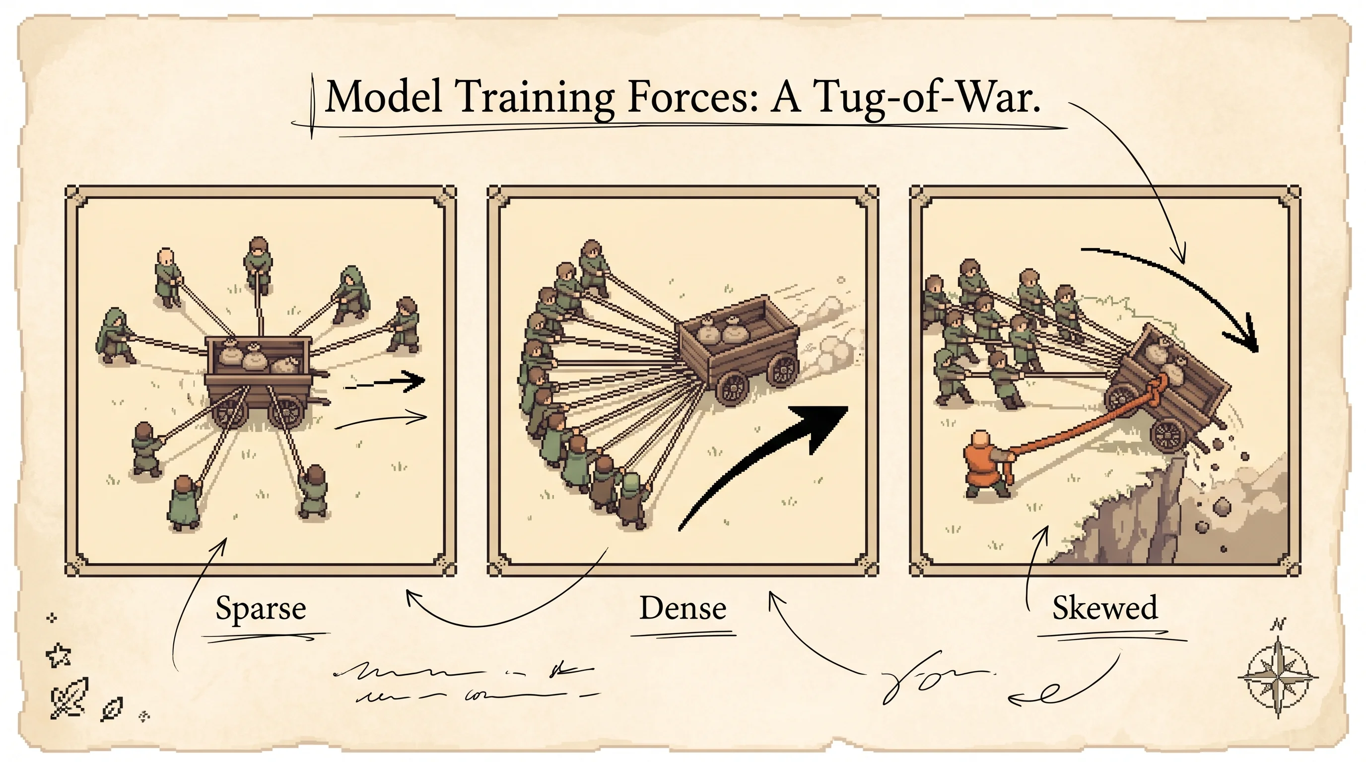
Imagine a little cart you want to push to a treasure chest, and a bunch of friends tied to it with ropes.
In the first game, your friends all pull in different directions, every which way. Most of the pulling cancels out, so the cart barely creeps forward. It's slow, but it never tips over, because no single friend can yank it somewhere silly. That's the careful way.
In the second game, all your friends pull the same general way, like a fan. The cart rolls far and fast. It's still safe, because they're spread out a little, so if one friend pulls a bit wrong it doesn't matter.
In the third game, almost everyone pulls gently, but one friend is a giant and grabs one rope and yanks as hard as a hundred friends, sideways, toward a cliff. The cart flies off the edge. To play this game safely, you have to tell the giant friend "you can only pull as hard as everyone else." Then the cart is fine again.
Each game is a way to teach the model. The careful slow one, the fast spread-out one, and the dangerous one with a giant that needs a rule to hold it back. Real ropes and carts aren't really there. The pulling is math that nudges a big pile of numbers inside the model, and the cart is the model getting better at its job.
For a high schooler
You've used autocomplete. It guesses your next word. A language model is a giant autocomplete, and after we build it we keep training it to guess better. Here's the one new idea for this section. Training means computing a gradient, which is just an arrow that says "nudge the model's numbers this way to make the good answer more likely." Every word in a training example produces its own little arrow, and the model adds them all up and takes one step.
The whole post is about the shape of that pile of arrows. Three shapes show up.
In RL, the model writes a full answer, and we only learn one thing at the end, whether it was right or wrong. That one bit gets smeared across every word. So most word-arrows are basically random noise. Here's the trick. When you average a huge pile of random arrows, they mostly cancel, and what survives is the small piece they all share, the part that actually points at "right." The step is tiny but you can trust it. Crank the batch size down in the simulation and watch this break. With only ten arrows the noise doesn't cancel, and the average points somewhere useless.
In SFT, every word comes with a "correct" answer to copy, so every arrow points the same general way, toward the teacher's style. Nothing cancels. You get a big step. It's safe because the arrows fan out a little across many different examples, so the model drifts toward all of them instead of slamming into one.
The dangerous shape is the third one. Take a math problem the model got wrong because it missed one key move. For the model, that move had maybe a 1 percent chance. For a teacher who already knows the answer, that same move is obvious, maybe 60 percent. The gap between 1 percent and 60 percent is enormous, so that single word produces an arrow about a hundred times bigger than a normal one. It doesn't cancel and it isn't spread out. One giant arrow drags the whole step toward a place the model didn't believe in, and the model breaks. The takeaway is that this method only works if you cap how big any one word's arrow can get.
For a college student
You should care about this because the order of operations in post-training, SFT first and then RL, is a convention almost everyone follows, and this post gives the real reason behind it. The reason is about which sampling distribution your method gets to compound with, and where that puts your performance ceiling.
Start with the two endpoints. SFT trains on completions from a fixed teacher. The defining property is that the sampling distribution is frozen at dataset-construction time. As the model improves, the data does not. Once the model gets close to the teacher's distribution, more SFT mostly memorizes, because the marginal example is no longer informative. So SFT's ceiling is roughly the teacher's quality.
RL is the opposite. The model samples its own rollouts, the gradient updates the policy, and the next batch comes from the improved policy. Improvements compound back into the sampling distribution. The ceiling isn't set by any data. It's set by whatever the verifier can grade.
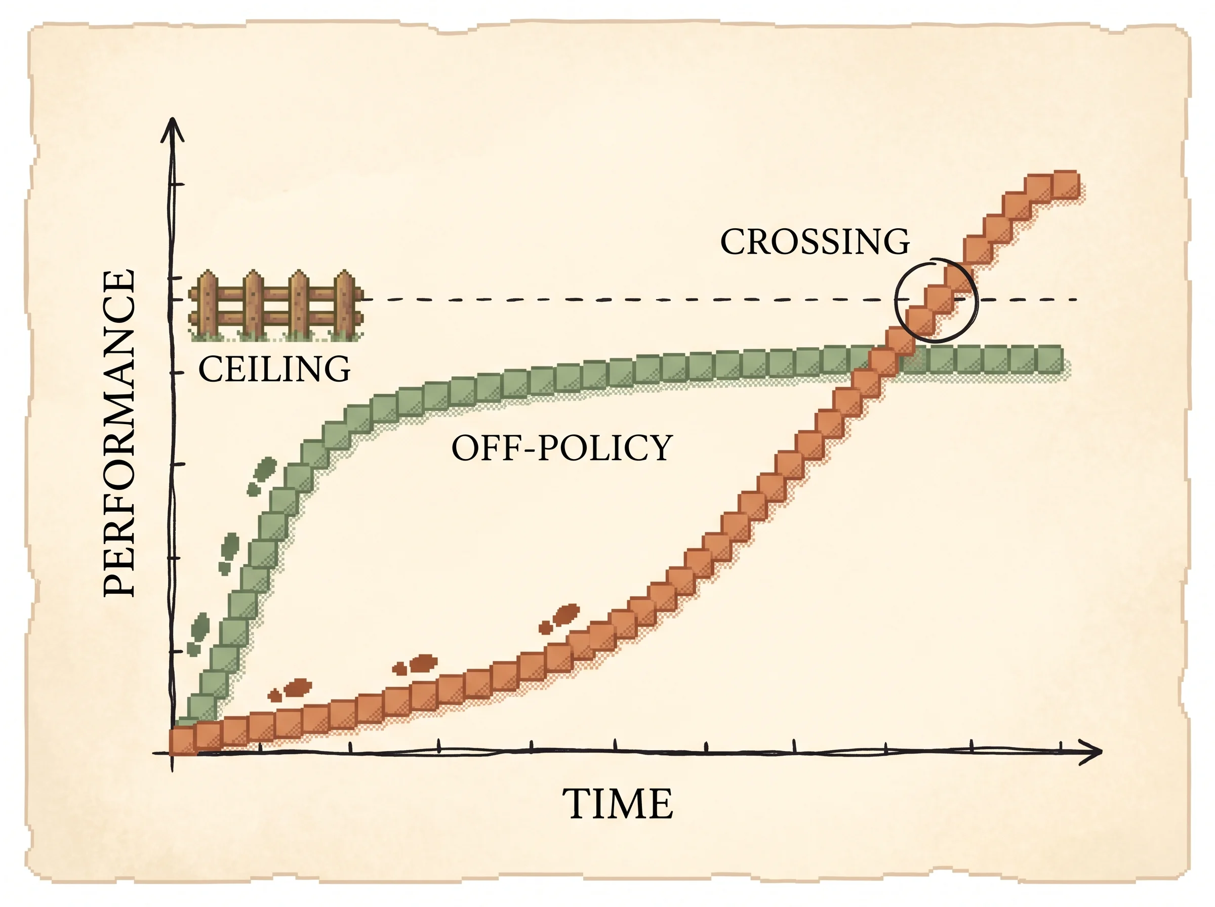
That gap creates a tipping point. When the model is far below the teacher and teacher data is cheap, SFT buys capability cheaply, because you're learning things you don't have from a source that does. As you approach the teacher, SFT examples get less informative, and the model's own lucky rollouts start producing genuinely new strategies that an RL gradient can extract. Past the tipping point, rollout compute is better spent on RL than on more SFT. That's the whole "SFT first, then RL" recipe in one sentence.
On-policy distillation sits between them. The model samples its own rollouts, so you get RL's compounding, but each token in the rollout is graded by a teacher through a per-token reverse KL.
grad J_OPD = E_{x, y ~ student} [ sum_t ( log pi_T(y_t | y_<t) - log pi_theta(y_t | y_<t) ) * grad log pi_theta(y_t | y_<t) ]The advantage at each token is "how much more the teacher prefers this token than the student does." It's dense, on-policy, and reverse-KL. The reported numbers are striking, roughly 9 to 30 times less compute than RL on AIME-style math benchmarks. The catch is that it needs a same-family teacher, because the per-token KL only makes sense when the teacher and student share a tokenizer and a similar training recipe. Without that match, the gradient ends up dominated by "the teacher would have phrased this differently" instead of "the teacher would have reasoned differently here."
The limitation falls out of that constraint. When you don't have a same-family teacher, you fall back to plain cross-family SFT, or RL, or the riskier self-distillation move in the next sections.
For an industry pro
The problem this solves for you is choosing where to spend post-training compute, and not torching a run by picking the wrong method at the wrong time.
Three methods, three operating envelopes. SFT is cheap and forgiving and gets you into a teacher's neighborhood fast, but it caps at the teacher and stops paying off once you're close. RL has no teacher ceiling and compounds, but the per-step signal is one bit of reward smeared across thousands of tokens, so it's slow and it wants large batches and patience to be stable. On-policy distillation is the best-of-both corner, RL's compounding with a dense per-token signal, and the post cites 9 to 30 times less compute than RL to reach a same-family teacher's level. Its hard requirement is a same-family teacher, meaning matched tokenizer and matched recipe, ideally the same base model at a bigger scale. Qwen3-32B teaching Qwen3-8B is the canonical case.
The failure mode to budget for shows up when you don't have that teacher and reach for self-distillation, where the model teaches itself using a hinted version of its own context. Conditioning the teacher on a hint or the answer sharpens its distribution. On most tokens the hinted teacher and the student agree, so the signal is small. But on a rare pivot token, the one key move the student missed, the teacher places huge mass where the student placed almost none, and that single token contributes on the order of a hundred times the loss of a typical one. Without a defense, the post reports performance collapse within about 100 steps. The defense is per-token KL clipping, capping how much any single vocabulary entry can contribute. Ship it on, or don't ship self-distillation.
The deeper win in same-family distillation isn't just cheaper sampling. It's on-policy state coverage. SFT trains under the teacher's states but you evaluate the model under its own, and that exposure-bias gap caps off-policy methods short of teacher quality on the real eval distribution. On-policy distillation trains on the model's own rollouts, so the gap never opens.
For a PhD candidate
The contribution here is framing, not a new algorithm. SFT, RL, OPD, and self-distillation are special cases of one token-level policy gradient, and a gradient-geometry analysis sorts them into a small taxonomy that predicts which ones are stable and why.
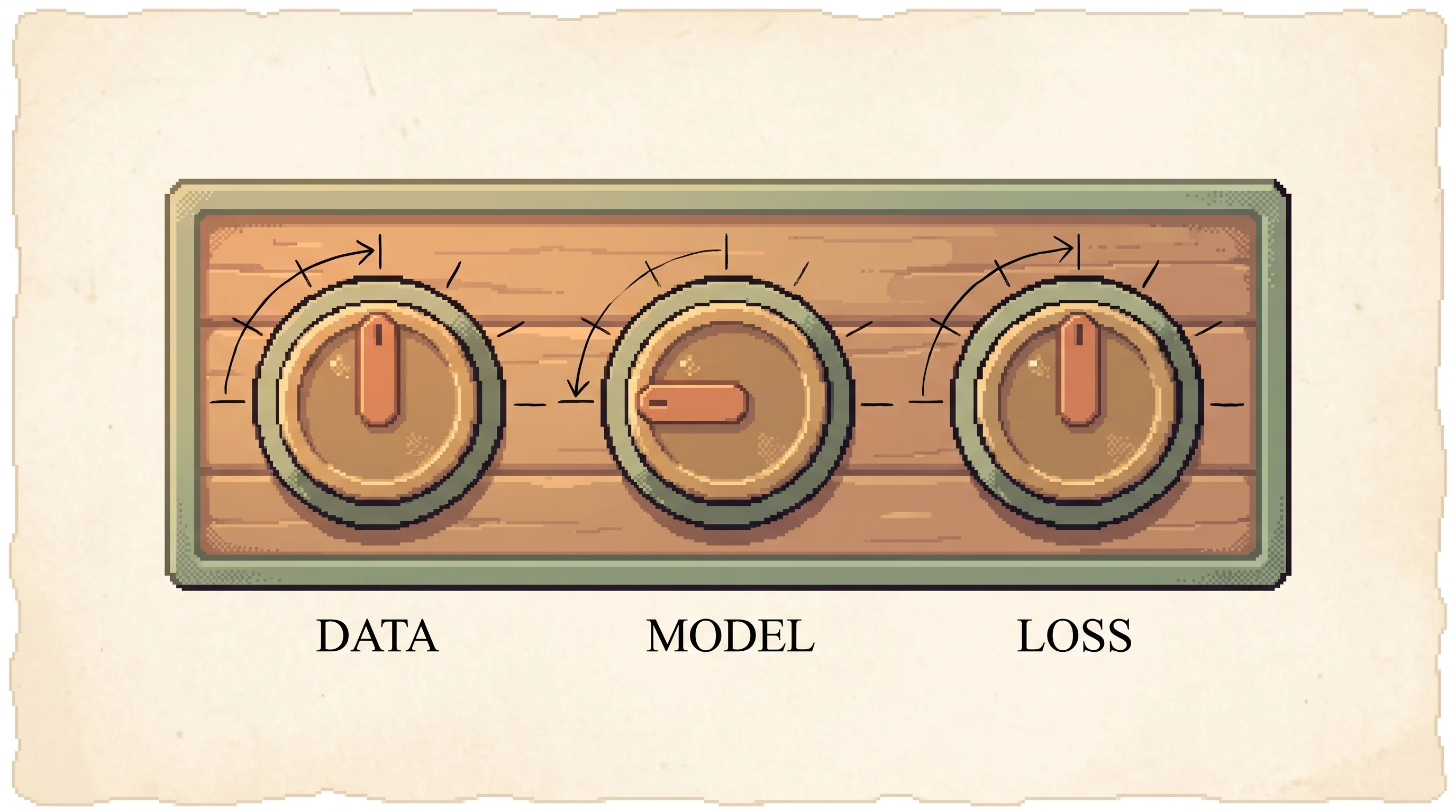
The meta-algorithm has three dials.
grad J(theta) = E_{x ~ D, y ~ mu_alpha} [ sum_t A_t(x, y) * grad log pi_theta(y_t | y_<t) ]

mu_alpha = alpha * pi_theta + (1 - alpha) * pi_data
A_t = lambda * [ log pi_T(y_t | c_T) - log pi_theta(y_t | y_<t) ] + (1 - lambda) * [ R(y) - b(x) ]
Alpha is how on-policy the sampling is. Lambda is how much of the per-token advantage comes from a teacher KL versus a sequence-level reward. The teacher policy pi_T is the third choice, which model conditioned on what context. SFT is alpha=0, lambda=1, with a degenerate point-mass teacher (the label). RL is alpha=1, lambda=0, teacher absent. OPD is alpha=1, lambda=1, external same-family teacher. OPSD is the same dial settings as OPD but with the teacher being the model itself conditioned on the ground-truth answer.
The geometry is where it gets sharp. Score each method on three axes, density, bias, and concentration. RL is sparse and unbiased, because most per-token advantages are noise whose mean is near zero by the group-baseline construction, so noise cancels and a small reward-correlated bias survives. That sparsity isn't purely a bug, it's the price of an unbiased estimator, and there's empirical support that RL updates are sparse in parameter space and modify small subnetworks. SFT is dense and biased toward the data, but diffuse, because the bias points slightly differently across many varied examples, giving a soft principal-components drift toward the data manifold rather than any one example. Same-family OPD inherits that diffuseness because the teacher is calibrated to the student's family.
OPSD is the unique cell with density, bias, and concentration at once. On a pivot token the reverse KL is roughly log(0.6/0.01) which is about 4.1 nats, while a typical token where both put around 0.3 contributes essentially zero. So one token carries about a hundred times the loss, and the resulting tug is neither cancelled like RL's noise nor spread like SFT's bias. That's why OPSD needs explicit defenses, per-token point-wise KL clipping or fixing the teacher to the initial policy, that the other methods don't.
Threats to validity worth probing. The geometry argument is illustrative rather than measured, the per-token-arrow picture is a useful intuition pump rather than a derived theorem, and the headline OPD compute numbers come from the cited reports, not from a controlled sweep in this post. The genuinely interesting open direction the post names is a teacher you can construct per task or online to be locally optimal for the current student, high reward and low KL, surgical rather than broadcast, so you sweep teacher quality against bias cleanly without needing a real fixed teacher.
For a peer researcher
Delta first. The move is to stop treating SFT, RL, and distillation as a menu and treat them as one estimator with a teacher choice and two scalar knobs, then read off stability from the gradient's geometry instead of from empirical lore.
The clean corners are where the statistics work without importance-sampling corrections. SFT (alpha=0, lambda=1) is distillation from a degenerate teacher, the data delta, and its safety comes not from the teacher being good but from the bias being averaged across many varied examples so it stays diffuse. RL (alpha=1, lambda=0) collapses the per-token signal to broadcast outcome reward, and the destructive-interference story is the whole reason large-batch low-learning-rate RL is robust despite each per-token gradient being mostly uninformative. OPD (alpha=1, lambda=1, same-family) gets dense and diffuse at once. OPSD shares OPD's dial settings, so the only thing that moves is pi_T, which is exactly why it can match OPD when it works and is where the failure mode is sharpest, the most distributionally aggressive teacher.
The author's own read is that interpolating alpha and lambda in the interior is probably a tangent, and the interesting axis of variation across the corners is the KL budget beta. The practically hard problem is teacher optimization, which is discrete (which model, which prompt, which hint) and doesn't decompose neatly into the gradient framing. The Lagrangian view, maximize expected reward gain minus beta times KL of teacher from student, traces a Pareto frontier where RL is the tangent at the origin (slope unbounded as KL goes to zero, gain scaling like sqrt(KL) locally) and the distillation methods are points further out. What would change the framing is a recipe that reaches the curve's interior without a real teacher and with compute-optimal learning at each point, which is the open question the post finds most interesting.
How it works
The problem and why the obvious moves fail. You've pretrained a model and want it better at a task you can grade. SFT copies a teacher, but its sampling distribution is frozen at dataset-construction time, so once the model nears the teacher it just memorizes and caps at the teacher's quality. Rejection-sampled SFT (filter teacher or student outputs for correctness, train on the survivors) shifts that ceiling up but doesn't change its shape, because the distribution is still pinned to whatever you filter. RL removes the ceiling by sampling the model's own rollouts so improvements compound, but its signal is one bit of reward per episode, which is slow.
The key idea. Read every method as the same token-level policy gradient with three dials, a sampling-policy mix alpha, an advantage-blend lambda, and a teacher choice pi_T. Then the question "which method is stable" becomes "what shape does this dial setting give the per-token gradient cloud." Three properties decide it, density (does each token get a signal or just the trajectory), bias (does the expected gradient point a fixed way), and concentration (is the signal spread across tokens or piled on a few).
The geometry, method by method. RL is sparse and unbiased. In a GRPO-style step, every token gets an advantage, the group baseline makes the advantages roughly zero-mean, and most token-arrows are noise that happened to share a trajectory with a reward. Average a large batch and the noise cancels, leaving the small consistent component along directions that correlate with reward. SFT is dense and biased but diffuse, every token gets a one-hot label so the arrows are dense and all point toward the data, but the data is varied so the bias spreads across many slightly different directions.
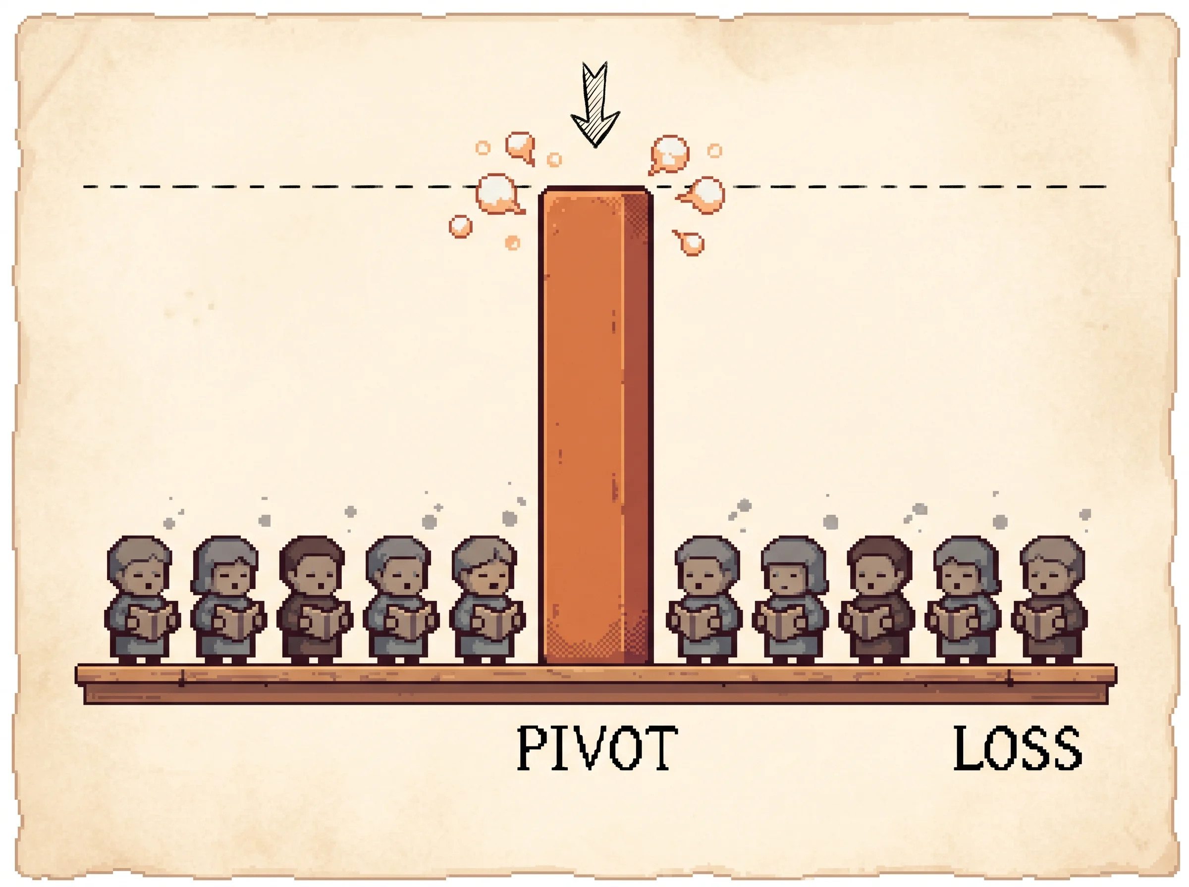
OPSD is the dangerous one. Consider a long math rollout the model got wrong because it missed one key move, the pivot token. For the model that token might have probability 0.01, but for a teacher conditioned on the answer it's 0.6, because once you know where the solution is going the right move is obvious. The per-token reverse KL between "student says 0.01" and "teacher says 0.6" is about log(0.6/0.01), roughly 4.1 nats, while a typical token contributes near zero. One token carries about a hundred times the loss, and that tug is neither cancelled nor spread. Load the OPSD: collapse preset to watch one pivot drag the averaged update past the safe radius.
The fix and the meta-algorithm. OPSD ships with per-token point-wise KL clipping, capping each vocabulary entry's contribution so a small subset of tokens can't dominate. Without it, the cited result is collapse within about 100 steps. Toggle the clip in the simulation and the update snaps back inside the safe radius. Pulling it all together, every method is the meta-algorithm above at a setting of alpha, lambda, and pi_T. The taxonomy then reads cleanly.
| method | density | bias | concentration | reliable when |
|---|---|---|---|---|
| RL | sparse | unbiased | diffuse (noise cancels) | large batches, patient |
| SFT | dense | toward data | diffuse (data is varied) | data is on-distribution |
| OPD (same-family) | dense | toward teacher | diffuse (teacher calibrated) | teacher is same-family |
| OPSD | dense | toward self+hint | concentrated on pivot tokens | aggressive clipping is in place |
Results with effect sizes. On-policy distillation is reported at roughly 9 to 30 times less compute than RL on AIME-style math, widening when teacher logprob calls parallelize. Self-distillation without the per-token clip collapses within about 100 steps, and the clip is what makes it usable.
Limitations and open questions. OPD needs a same-family teacher, a hard constraint. The gradient-geometry argument is an intuition pump, not a measured result. The open direction is constructing a teacher per task or online to be locally optimal for the current student, so you can sweep teacher quality against bias without a fixed external teacher.
My assessment
The strongest thing here is the reframe. Treating four methods as one gradient with three dials turns a pile of folklore ("SFT first, then RL," "distillation is cheaper," "self-distillation is unstable") into one picture you can reason about. The density-bias-concentration taxonomy earns its keep, because it predicts the OPSD failure from first principles, the pivot token is concentrated, concentrated dense bias has neither RL's cancellation nor SFT's spread to save it, so it must be clipped. That's a real explanation, not a description.
Where I'd push back is on how much the geometry is doing versus asserting. The per-token-arrow story is a model of the gradient, and the post is honest that it's illustrative, but the leap from "RL updates are observed to be sparse in parameter space" to "destructive interference is the mechanism" is suggestive rather than shown. The compute numbers come from cited reports, so they inherit those papers' conditions. None of that dents the framing, which is the contribution.
The part I find most interesting is the part the author flags as unsolved. If you could construct a teacher per task or online that's locally optimal for the current student, high reward and low KL, you'd get the interior of the Pareto curve between distillation and RL without needing a fixed external teacher, with compute-optimal learning at every point. That's the move that would make "pick your beta, then build the best teacher for it" a real algorithm rather than a diagram, and it's the right open question to be chasing.