High-Dimensional Continuous Control Using Generalized Advantage Estimation
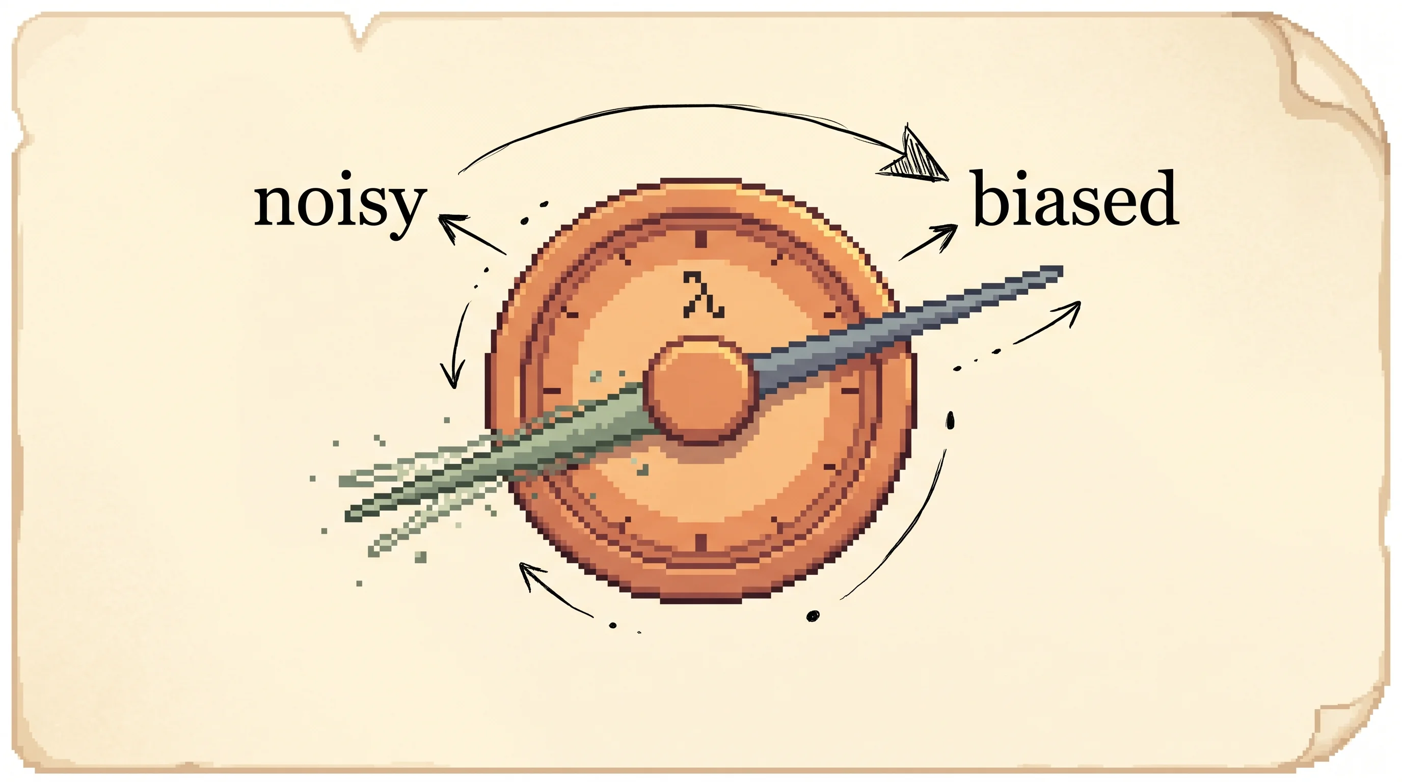
One dial slides a reinforcement-learning agent's reward estimate between a noisy-but-honest guess and a calm-but-biased one, and the sweet spot in the middle teaches simulated robots to run and stand up.
Read at your level
Start where you're comfortable and climb as far as you like.
- For a 5-year-old
- For a high schooler
- For a college student
- For an industry pro
- For a PhD candidate
- For a peer researcher
Executive summary
An agent that learns by trial and error needs to know, for each move it made, whether that move was better or worse than usual. That number is the advantage, and you can't see it directly, so you estimate it from the rewards that follow. Estimate it from the full stream of future rewards and your guess is honest but jumpy, because a thousand later flukes drown out the one move you're judging. Estimate it from a single step plus a learned value guess and it's calm but slanted, because your value guess is wrong early on. Generalized advantage estimation puts one dial, called lambda, between those two extremes. It blends a one-step guess, a two-step guess, a three-step guess, and so on, trusting each longer one a little less. Turn the dial and you trade jumpiness for slant. The authors found the best setting sits near the calm end, around 0.95, and with it they trained neural-network policies to make simulated robots run on two legs, run on four, and stand up off the ground, all from raw joint readings. The cost is that lambda only helps when paired with a decent value guess, and the whole thing still burns through one to two weeks of simulated robot time per task.
Try it
Load the One-step on a broken V preset, watch the bias light turn red and the return stall short of the dashed ceiling, then drag the lambda dial up toward 1 and watch the bias fall and the climb restart. Then load Monte Carlo, where lambda sits at 1 with a wrong value function, and notice the bias light stays green while the variance readout runs high and the curve jitters.
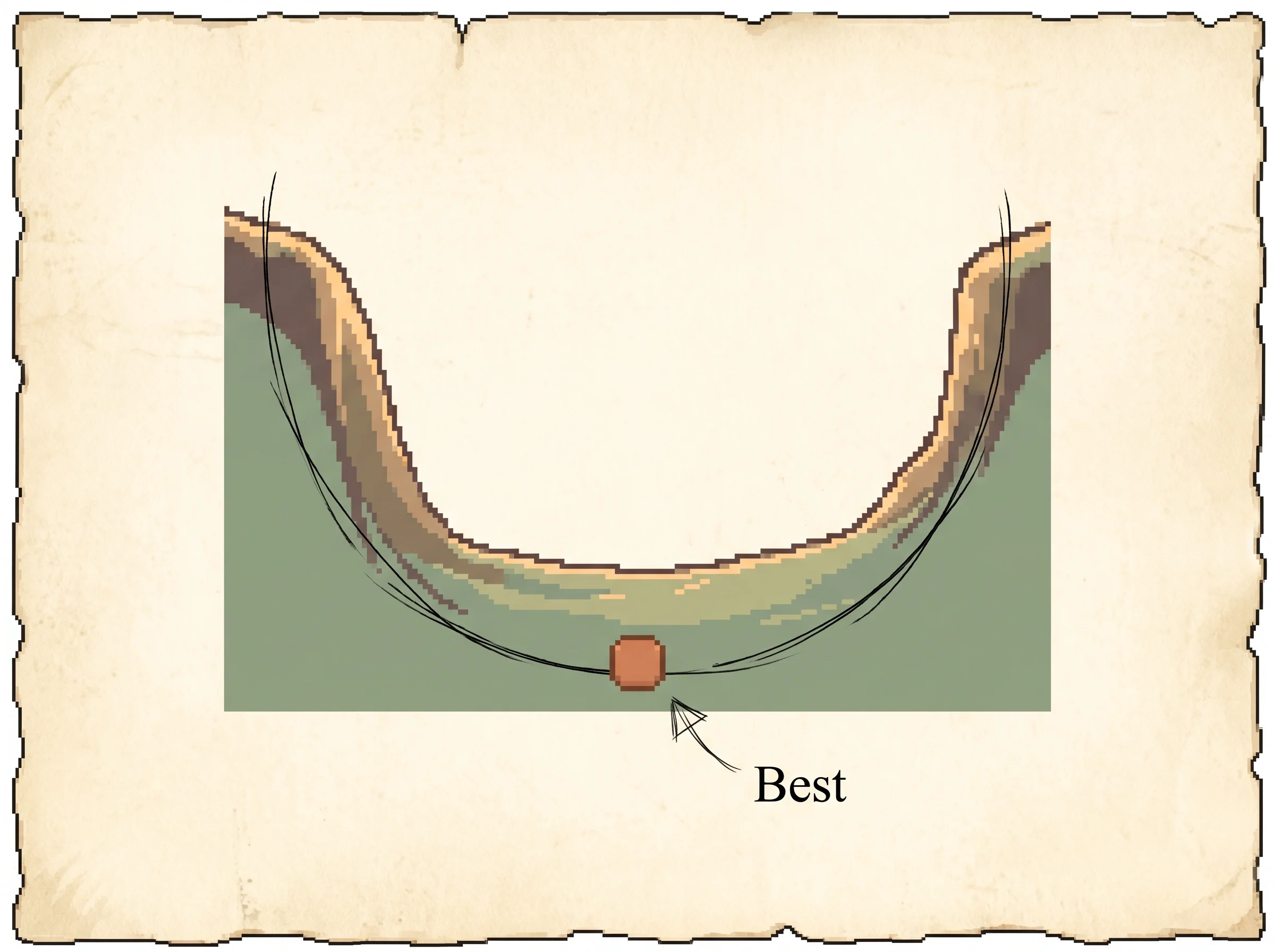
The paper's sweet spot. With a good value function and lambda at 0.96, the advantage estimate has low bias and low variance. Press play and watch the return climb fast and smooth to optimal while the bias light stays green.
Run a few steps to draw the return and bias curves.
Click a cell to read its value estimate, its move probabilities, and each move's true advantage. The longest arrow is the policy's favored move; clay-orange marks it. Greener cells hold more value.
Reach optimal or flip a control to start the log.
A softmax policy on a 5 by 5 gridworld with a goal worth +1 and a trap worth −1. Each step samples a batch of episodes, estimates the advantage at every visited step with GAE(gamma, lambda) = the exponentially-weighted sum of TD residuals, and takes one policy-gradient ascent step. The bias readout is the angle between the estimator's expected gradient and the true gradient, computed on the side only to score it. It sits near zero at lambda 1 for any value function, and grows as lambda shrinks under a wrong value function. This stands in for the paper's trust-region update and neural-network value function with one plain ascent step on a solvable grid. Each preset starts from a fixed rollout seed so the same preset always produces the same run; loading a preset resets it.
For a 5-year-old
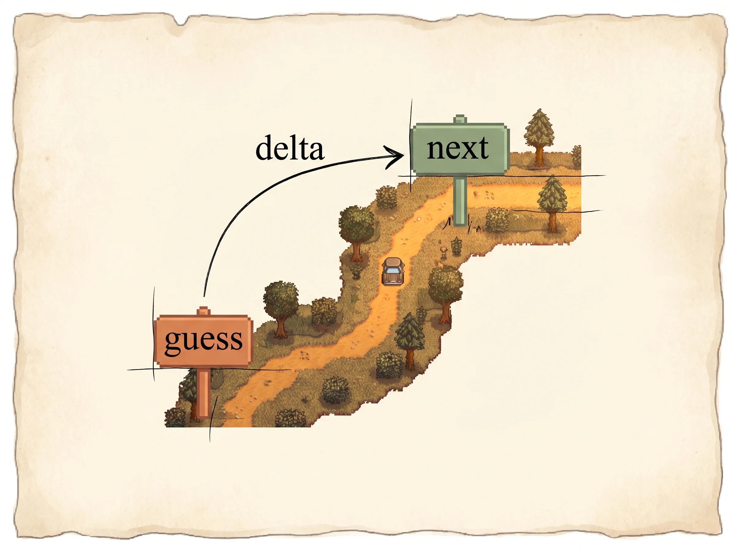
Imagine you're in a car on a long drive to grandma's house. You want to guess how many more minutes until you get there. There are two ways to guess.
One way is to wait until you actually arrive, then count how long it really took. That guess is always right. But you have to sit through the whole drive before you learn anything, and every drive is a little different, so the number jumps around a lot. Today there was traffic. Tomorrow there wasn't.
The other way is to peek at the little screen on the dashboard that says "20 minutes left." That guess comes right now, and it doesn't jump around. But the screen is often wrong, especially at the start of the trip.
So here's the trick. You don't pick just one way. You mix them. You listen to the screen a little, and you wait and see a little, and you blend the two. There's a dial that says how much to trust the screen versus how much to wait and see. If you spin the dial just right, your guesses stop jumping around so much and they stop being so wrong. The car learns the fastest way to grandma's house.
The car isn't really guessing minutes. It's a robot guessing whether each little wiggle of its legs was a good idea. But the dial is real, and finding the right spot on the dial is the whole idea.
For a high schooler
You've used a maps app that shows your arrival time. The number updates as you drive. Reinforcement learning has the same problem in reverse. A robot makes a move, then a bunch of stuff happens, and it has to figure out whether that one move was good. The trouble is telling apart the effect of that move from everything that came after.
Here's the one new word for this section. The advantage of a move is how much better that move was than the robot's usual move from the same spot. A positive advantage means do more of that. A negative advantage means do less. The robot can't measure the advantage directly, so it estimates it from the rewards that come later.
There are two honest ways to estimate it, and both have a flaw. The first is to add up every reward from that move to the end of the episode. That sum is unbiased, meaning it's right on average. But it swings wildly, because hundreds of later events, most of them nothing to do with the move you're judging, pile into the sum. The second way is to look one step ahead and lean on a learned guess of how good the next spot is, called the value. That's steady, but the value guess is wrong while the robot is still learning, so the estimate is slanted.
Now the worked example. Say a move's true advantage is +2. The full-sum method might report +9 today and −4 tomorrow, averaging to about the right answer but never landing on it. The one-step method might report +0.5 every time, calm but consistently too low because the value guess is off. Neither is good enough alone.
Generalized advantage estimation blends them with a dial called lambda, a number from 0 to 1. Near 0, you trust the calm one-step guess. Near 1, you trust the jumpy full sum. In between, you get a mix that's both steadier than the full sum and less slanted than the one-step guess. Spin the dial to the right spot and the robot learns much faster.
For a college student
You should care about this because it's the variance-reduction trick that made deep reinforcement learning work on hard control problems, and it's a direct ancestor of the advantage estimates inside PPO, which is what trained the first useful RLHF language models.
The setup is policy gradient. You have a policy pi_theta(a | s), a distribution over actions given a state, with parameters theta. You want to maximize expected total reward. The policy gradient theorem says you can climb that objective with
g = E[ sum_t Psi_t * grad_theta log pi_theta(a_t | s_t) ]where Psi_t is some signal telling you how good action a_t was. The lowest-variance honest choice for Psi_t is the advantage A(s_t, a_t) = Q(s_t, a_t) - V(s_t), which measures exactly how much better the action was than the policy's default. You don't know the advantage, so you estimate it.
The building block is the TD residual. Define a value function V(s), your current guess of how much reward follows state s. Then
delta_t = r_t + gamma * V(s_{t+1}) - V(s_t)is the one-step surprise: the reward you actually got plus your guess for the next state, minus your guess for this one. gamma is the discount, between 0 and 1, that shrinks rewards the further off they are.
If V is exact, delta_t is already an unbiased estimate of the advantage. It usually isn't exact, so a single delta_t is biased. The fix is to look further ahead. Sum k of these residuals and you get a k-step estimate that leans less on V and more on real rewards. The one-step estimate trusts V the most; the infinite-step estimate ignores V except as a baseline and is the full discounted return minus V(s_t).
GAE doesn't pick one k. It takes an exponentially-weighted average of all of them, weighted by lambda^k. The whole sum collapses to a clean formula:
A_hat_t = sum_{l >= 0} (gamma * lambda)^l * delta_{t+l}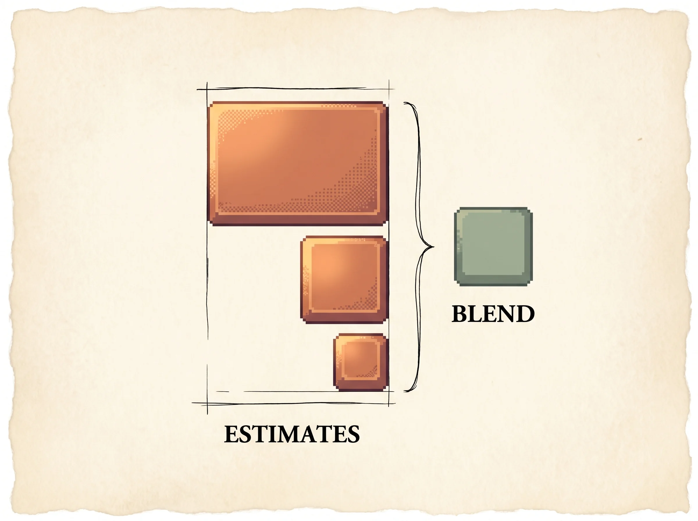
Read the two ends. At lambda = 0, the sum is just delta_t, the one-step estimate: low variance, biased unless V is exact. At lambda = 1, the V terms telescope away and you're left with the full discounted return minus V(s_t): unbiased for any V, high variance. The dial in between trades the two.
Here's the worked path the simulation runs. Start with a value function set to zero everywhere, the worst possible. At lambda = 0 the estimate is r_t - 0, a single reward with no idea of the future, so it's heavily biased and the policy stalls. Drag lambda to 1 and the estimate becomes the full return, which is honest even though V is garbage, so the policy starts climbing again. That swing is the entire point of the dial.
The limitation is that lambda earns its keep only next to a half-decent value function. With a perfect V you'd want lambda = 0 for zero variance. With a useless V you're forced toward lambda = 1 and pay full variance. The interesting regime, and where the paper lives, is a learned V that's roughly right, where a middle lambda beats both ends.
For an industry pro
The problem this solves is sample efficiency in policy-gradient RL. Vanilla REINFORCE estimates the gradient from full-episode returns, and the variance of that estimate grows with the horizon, so on a long-horizon control task you need an absurd number of rollouts before the gradient points anywhere useful. GAE cuts that variance by leaning on a learned value function, without committing to the heavy bias of a pure one-step actor-critic.
What it costs to deploy. You need a second network, the value function, trained alongside the policy, plus two new scalars to tune, gamma and lambda. The paper's defaults are a strong starting point: gamma in [0.99, 0.995] and lambda in [0.95, 0.98]. The good news is the result is not knife-edge sensitive. There's a broad basin of decent settings, and you'll feel the cliff only at the extremes.
The expected improvement over a full-return baseline is large on long-horizon tasks and small on short ones, because variance is the thing being cut and variance scales with horizon. On the paper's 3D biped, the value-function runs reach a stable gait while the no-value-function baseline crawls.
The failure mode to plan around is a bad value function paired with a low lambda. That combination doesn't just slow learning, it biases the gradient toward the wrong answer, and more data won't save you because bias doesn't average out. If your value network is undertrained or your reward is hard to predict, push lambda up toward 1 and eat the variance until the value network catches up. The simulation makes this concrete: a zeroed value function at lambda 0 stalls, and the only fix is the dial, not more episodes.
For a PhD candidate
The contribution is twofold and worth separating. First, a clean justification and analysis of the exponentially-weighted advantage estimator, GAE(gamma, lambda), which had appeared in the online actor-critic work of Kimura and Kobayashi and of Wawrzynski but lacked a general bias-variance account that covers the batch setting. Second, the use of a trust-region method for the value function, mirroring TRPO on the policy side, which the authors find a robust way to fit large value networks.
The framing that pays off is the two-discount picture. GAE introduces lambda as a second, "steeper" discount applied on top of gamma, and the paper shows via the reward-shaping construction of Ng et al. that GAE(gamma, lambda) is exactly the gamma-lambda-discounted sum of Bellman-residual shaped rewards, where the shaping potential is V. That reframing is why the two parameters play different roles. Gamma sets the scale of the value function V^{pi,gamma} and controls bias even when V is exact, because it defines which problem you're solving. Lambda introduces bias only to the extent V is inaccurate. So the empirically observed gap, best lambda well below best gamma, falls out: lambda's bias is gated by value-function error, gamma's isn't.
The methodological choices reward scrutiny. The value function is fit with a trust-region step, constraining the average KL between the old and new conditional Gaussian over values rather than taking unconstrained Gauss-Newton steps, which the authors argue avoids overfitting the most recent batch. The policy update is TRPO, held fixed across conditions so the experiments isolate the effect of gamma and lambda. One subtle honesty point the paper makes: the policy update at iteration i uses the value function from iteration i, not i+1, because fitting the value first would let an overfit V drive the Bellman residuals to zero and zero out the gradient.
Threats to validity worth probing. The locomotion gains rest on MuJoCo simulation with a specific reward shaping (a forward-velocity term, a control-cost term, and a survival bonus), and the survival bonus is doing quiet work to stop the policy from ending episodes early. The lambda sweep is run at a fixed gamma, so the joint surface is sampled coarsely. And the claim that lambda's bias is small "for a reasonably accurate value function" is supported empirically rather than bounded, which is the obvious open problem.
For a peer researcher
The delta against prior actor-critic work is that GAE gives a single knob spanning the whole bias-variance frontier, from the high-bias one-step estimator at lambda 0 to the unbiased high-variance Monte Carlo estimator at lambda 1, with a clean closed form and a batch-setting analysis, rather than a fixed eligibility-trace choice baked into an online update. The delta against TRPO alone is the variance reduction that makes long-horizon 3D control tractable, plus the trust-region value-function fit.
The choices read as deliberate tradeoffs. Lambda below 1 buys variance reduction by accepting bias proportional to value-function error, which the reward-shaping analysis pins down via the response function chi(l): a discount gamma below 1 drops terms beyond l about 1/(1-gamma), and that's harmless exactly when the response function decays fast, which a good V enforces by collapsing the temporal spread. So the bet is that an approximate V partially reduces the response horizon, and lambda then cuts the residual long-delay noise. That's the conceptual core, and it's why this generalizes past locomotion.
What would change my mind on the central claim. If a learned value function good enough to drive lambda toward 0 were cheap to obtain, the intermediate-lambda story would weaken into "just fit V better." It isn't cheap, which is why the dial matters. The honest soft spot is the absence of a bound relating value-function error to advantage-estimation bias, which the authors flag as future work, and which would turn the lambda choice from a sweep into a principled setting tied to a measurable value-function error metric.
How it works
The problem and why prior approaches failed. Policy gradient methods optimize expected reward directly and work with any differentiable policy, which is why they scale to neural networks. The catch is the gradient estimate. With full-episode returns it's unbiased but its variance grows with the horizon, because the effect of one action gets confounded with every action before and after it. Actor-critic methods swap the return for a value function to cut variance, but they introduce bias, and bias is the worse poison: even with infinite data, a biased gradient can converge to a non-optimal policy or fail to converge at all. Prior work picked a point on this spectrum and lived with it.
The key idea. Estimate the advantage with an exponentially-weighted average of all the k-step estimates, controlled by one parameter lambda. The building block is the TD residual delta_t = r_t + gamma * V(s_{t+1}) - V(s_t), and the estimator is
A_hat_t^{GAE(gamma, lambda)} = sum_{l >= 0} (gamma * lambda)^l * delta_{t+l}This single formula spans the whole frontier. Lambda 0 gives delta_t, the steady biased one-step estimate. Lambda 1 gives the full discounted return minus the baseline V(s_t), unbiased for any V. Everything useful lives in between.
Methodology. The full loop is short. Run the current policy to collect a batch of timesteps. Compute delta_t at every step using the current value network. Sum them with the (gamma * lambda)^l weights to get A_hat_t. Form the policy gradient estimate and take a TRPO step. Refit the value network with its own trust-region step. Repeat.
for each iteration:
    run policy pi to collect N timesteps
    delta_t = r_t + gamma * V(s_{t+1}) - V(s_t)        # at all t
    A_hat_t = sum_l (gamma * lambda)^l * delta_{t+l}    # at all t
    update policy with a TRPO step using A_hat
    refit V with a trust-region regression step
The networks are plain feedforward nets with three hidden layers (100, 50, 25 tanh units), one for the policy mapping state to a distribution over joint torques, one for the value function with a scalar output. No hand-crafted features, no model of the dynamics, raw kinematics straight to torques.
Results with effect sizes. On cart-pole, the fastest learning came from intermediate values, gamma in [0.96, 0.99] and lambda in [0.92, 0.99], with both extremes clearly worse. On 3D bipedal locomotion (33 state dimensions, 10 actuators), the best settings were gamma in [0.99, 0.995] and lambda in [0.96, 0.99], reaching a fast, smooth, stable gait after about 1000 iterations, while the no-value-function baseline lagged far behind. The same recipe learned quadrupedal running and learned a biped to stand up off the ground. The simulated experience for the biped tasks works out to one to two weeks of real time.
Limitations and open questions. Lambda reduces bias only when V is reasonably accurate, so the method inherits the value function's quality. The authors give no bound tying value-function error to advantage-estimation bias, leaving the lambda choice to a sweep. Sample cost is still high in absolute terms. And the open directions they name are setting gamma and lambda adaptively, finding an error metric for the value fit that matches the policy-gradient error, and sharing features between the policy and value networks.
My assessment
The authors got the central thing right, and the field has voted with its feet. The GAE advantage estimate is the default inside PPO, which became the workhorse of applied RL and the engine behind the first round of RLHF-tuned language models. The reason it stuck is that it solved a real, painful problem (long-horizon variance) with one interpretable knob and a closed form that costs almost nothing to compute. That combination of cheap, general, and tunable is what makes a method survive.
The cleanest part of the paper is the reward-shaping reframing. Showing that GAE is the gamma-lambda-discounted sum of Bellman-residual shaped rewards is what turns lambda from a heuristic eligibility-trace parameter into something you can reason about, and it's what explains why best-lambda sits below best-gamma. That insight has aged better than the locomotion results themselves, which were impressive in 2016 and have since been dwarfed.
Where the paper left the door open is exactly where it admitted it would. There's still no principled way to set lambda from a measurable property of the value function, so in practice everyone sweeps it or copies the paper's defaults. The honest framing of that gap, rather than papering over it, is part of why the work reads as solid a decade on. The bet underneath it all, that an approximate value function shrinks the temporal reach of credit assignment enough that a steeper discount can safely cut the rest, turned out to be exactly the right bet for the deep RL era.