Simple Statistical Gradient-Following Algorithms for Connectionist Reinforcement Learning
A learner can climb toward more reward by doing more of whatever random move just beat its own recent average, and although it never measures a slope or maps its world, averaging these blind tweaks over many tries points it in the exact uphill direction of expected reward.
Read at your level
Start where you're comfortable and climb as far as you like.
- For a 5-year-old
- For a high schooler
- For a college student
- For an industry pro
- For a PhD candidate
- For a peer researcher
Executive summary
You want a learner to get better at a task, and all you can give it back is a single number, the reward, that says how well it just did. The hard part is that the learner acts at random and never sees why a reward was high or low, so it can't tell which of its choices to thank. The old fix was to build a model that predicts reward and then differentiate that, which means learning a whole second thing first. Ronald Williams' 1992 paper skips the model. Each random unit keeps one small local quantity, the characteristic eligibility, which measures how the unit's actual output deviated from its average and pins that deviation on each weight. After every trial the learner nudges each weight by the reward, minus a running average, times that eligibility. Williams proves the surprising part. Average those noisy little nudges over many trials and they point exactly along the gradient of expected reward, so the learner climbs toward more reward without ever computing or storing a gradient. He calls the whole family REINFORCE, derives the rule for coin-flip units and for Gaussian units that learn how widely to explore, extends it to delayed reward, and shows it plugs into backpropagation. The cost is that the per-trial signal is noisy, so learning is slow and can settle on a local peak, and there's no proof it always converges. That update is the seed of every policy gradient method that came after, including the ones that tune today's language models.
Try it
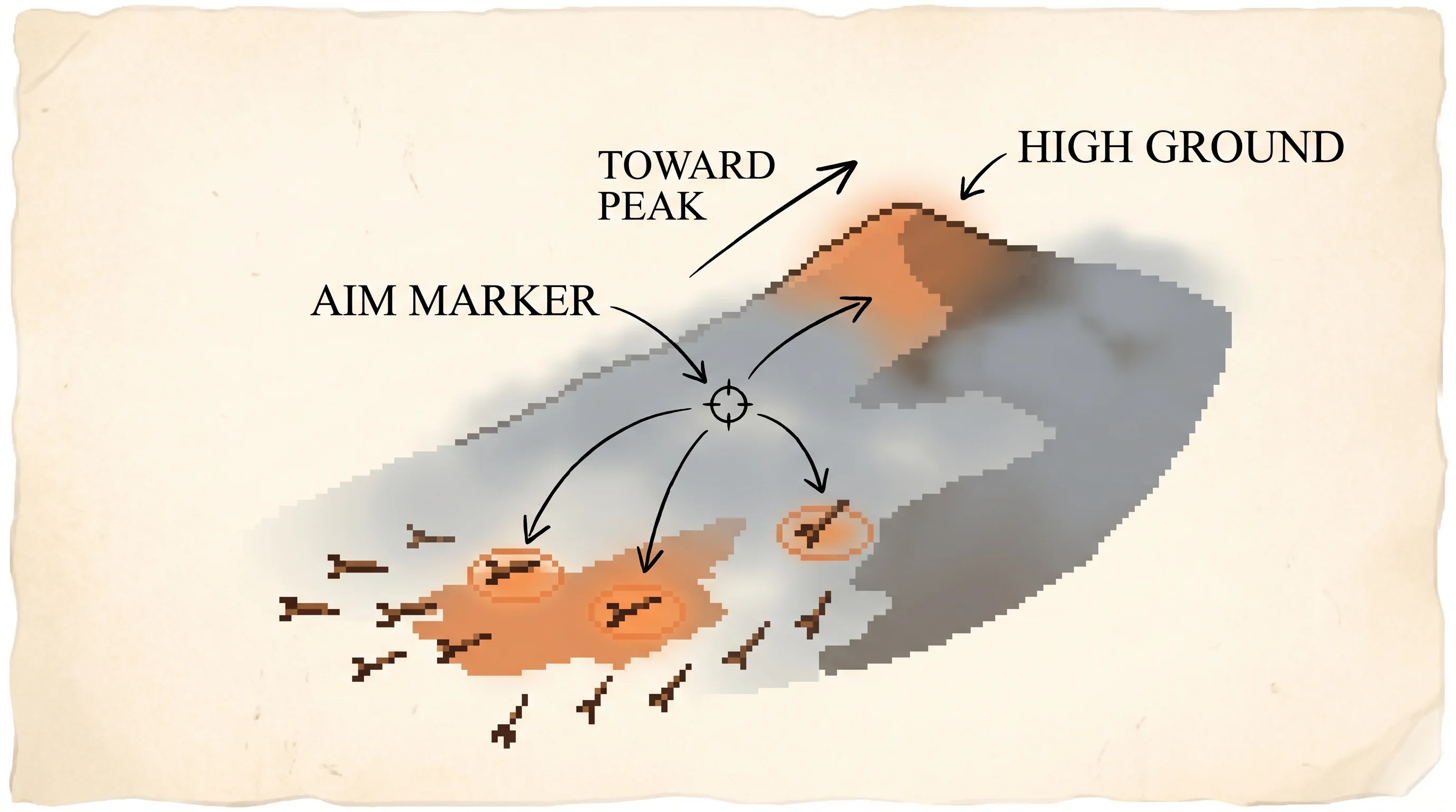
Load Climb the hill and press play. A cloud of random tries scatters around the aim, drifts uphill batch by batch, and its dashed ring tightens onto the bright peak. Watch the orange arrow, the unit's averaged step, swing into line with the faint dashed arrow, which is the true uphill direction it can't see. Then load Trapped on a lesser peak, let it settle onto the small hill, and click far out on the tall hill's slope to drop the aim there and watch it climb the bigger one. Switch the baseline to none on the No baseline, noisy climb preset and watch the spread balloon and the climb lurch, then switch it back to reinforcement comparison and watch the same run steady.
One Gaussian unit on a single hill it cannot see. Run it and watch the cloud of tries drift uphill while its spread tightens onto the peak. The reward climbs, the averaged step lines up with the true gradient, and the optimal light turns on.
Run a few batches to draw the reward curve.
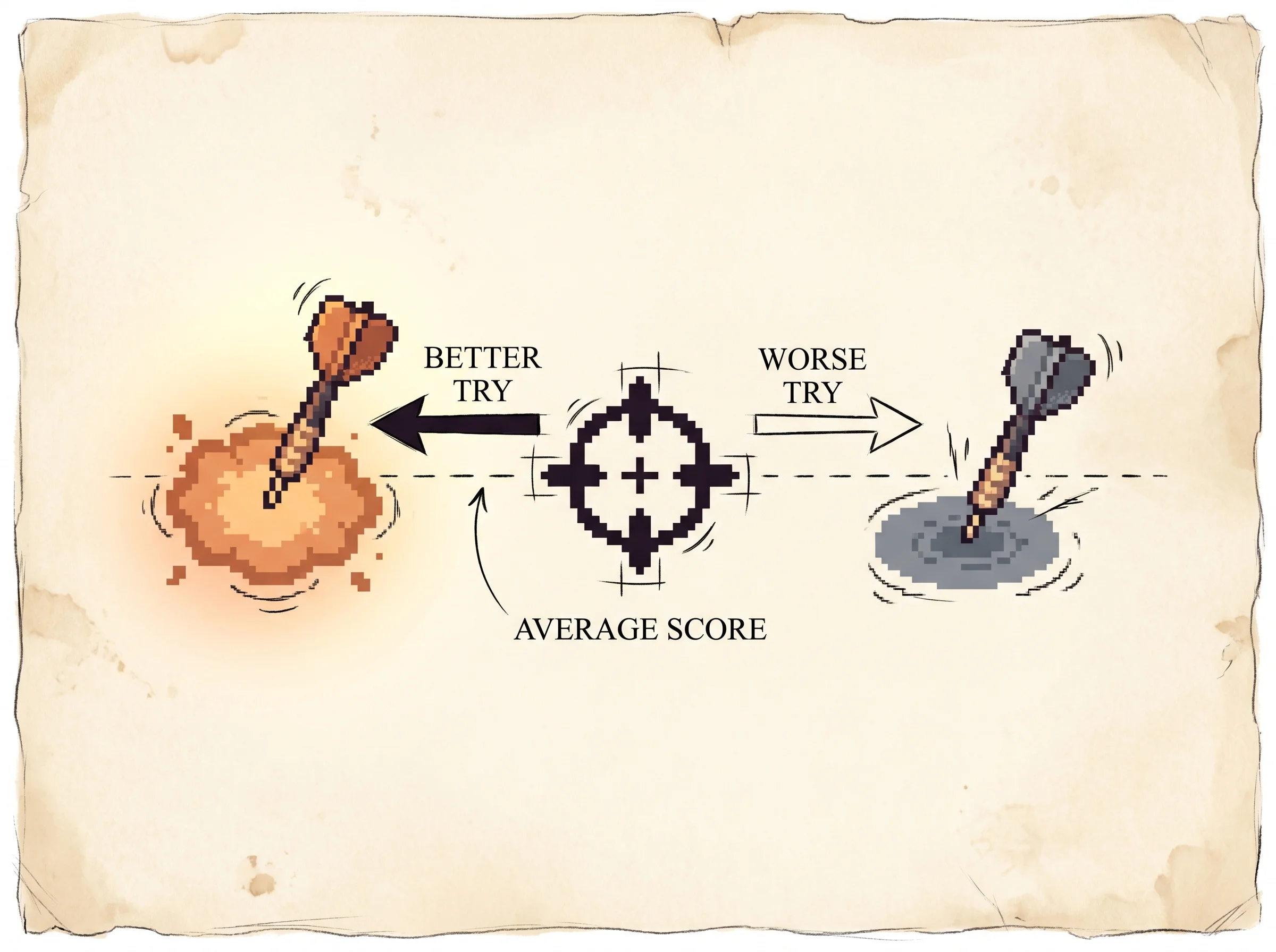
Click the landscape to drop the aim anywhere. Hover a try to read its score. Filled orange tries beat the baseline and pull the aim; hollow slate tries fall short and push it away.
Reach a peak or flip a control to start the log.
Each batch draws 24tries from N(aim, sigma squared), scores them on the hidden landscape, and applies the paper's averaged update, Δμ = α(r − b)(y − μ) and the matching rule for sigma. The orange arrow is the unit's averaged step; the faint dashed arrow is the true gradient of expected reward, computed separately only to check that the averaged step aligns with it (Theorem 1). The ring on the heatmap marks the tallest hill, which the unit never sees. The run uses a fixed seed; Reset replays the same trajectory.
For a 5-year-old
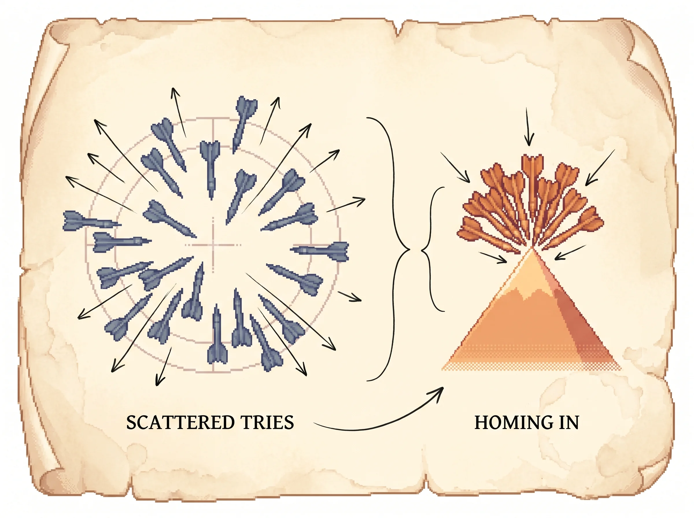
Imagine throwing soft beanbags at a hill, but it's so foggy you can't see the top. You toss a whole handful at once. A friend tells you which bags landed on high ground and which landed low. You don't get to see the hill and you don't get a map. You just lean your next throws a little toward where the high ones landed and a little away from where the low ones landed.
Toss, lean, toss, lean. Bit by bit you creep up the hill you can't see.
When you're lost down at the bottom you throw your bags far and wide, so a few might land somewhere good and show you the way. Once you're near the top and scoring well, you throw them close together, right where it's working.
Nobody really shouts "higher" or "lower." The thrower just remembers how good its throws usually score, and checks each new throw against that. A throw that beats the usual score pulls the aim toward it. A throw that falls short nudges the aim away. That little comparison is the whole trick.
For a high schooler
Think about how you got good at a game by playing it, not by reading the manual. You tried things, some worked, you did more of those. This is that idea, written down so a machine can do it.
Here's the setup. The learner makes a random choice every turn. Picture it flipping a weighted coin, where the weight is how likely it is to say yes. After it chooses, the world hands back one number, the reward, and nothing else. No explanation. The learner has to get better using only that number.
The rule is short. Do more of what beat your average, less of what fell short. To make that exact, the learner keeps a running average of its recent reward, call it the baseline. Each turn it compares the reward it just got to that baseline. If the reward came in above the baseline, it shifts its coin to make the choice it just made more likely. If the reward came in below, it shifts the coin the other way.
Here's a worked example with numbers. Say the coin currently lands "yes" 40 out of 100 times, so its chance is 0.4. This turn it happened to land yes, and the reward was 1, while its baseline (its usual score) is 0.3. The reward beat the baseline, and it landed yes, so it bumps the chance of yes up, maybe to 0.45. Next time it's a bit more likely to do the thing that just worked. Had the reward come in at 0.1, below the baseline, it would have pushed the chance of yes down instead.
The amount it shifts has a clean form. It's the reward-above-baseline times how surprising the choice was. A "yes" when yes was already near-certain barely moves anything, because there was nothing to learn. A "yes" that was a long shot moves the chance a lot. That "how surprising was my own output" number is the heart of the method.
Any single turn is noisy, because the reward was partly luck. But do this thousands of times and the lucky turns cancel out, and what's left is a steady drift toward choices that pay more. The learner ends up climbing toward reward it could never see directly.
For a college student
The setting is one trial of an associative reinforcement task. The learner reads an input, produces an output y drawn at random from a distribution it controls, and receives a scalar reward r. For a single Bernoulli unit the output is 0 or 1, and the unit sets the probability of a 1 by squashing a weighted sum of its inputs:
p = f(s),   s = sum over j of w_j x_j,   f = logistic
y = 1 with probability p, else 0
The thing you actually want to maximize is the expected reward, averaged over the unit's own randomness and the environment's:
J(W) = E{ r | W }You can't differentiate r directly, because r depends on a random draw and on an environment you don't model. Williams' move is the likelihood-ratio identity, sometimes called the log-derivative trick. Write the expected reward as a sum over possible outputs, then differentiate:
d/dw E{r}  =  d/dw  sum_y  g(y) r(y)
           =  sum_y  r(y)  dg/dw
           =  sum_y  r(y)  g(y)  (d ln g / dw)      since dg/dw = g * d ln g/dw
           =  E{ r * (d ln g / dw) }
Read the last line carefully, because it's the whole paper. The gradient of expected reward equals the expected value of reward times d ln g / dw. That second factor, the gradient of the log-probability of the output the unit actually produced, is what Williams names the characteristic eligibility. It's a local quantity each unit can compute from its own output and input alone. So one sample of r * (d ln g / dw) is an unbiased estimate of the true gradient. You never form the gradient or store anything to form it. You just multiply the reward you got by a number the unit already knows.
The REINFORCE update adds a baseline b and a learning rate alpha:
delta w = alpha (r - b) (d ln g / dw)Subtracting a baseline doesn't bias the estimate, as long as b doesn't depend on the current output. The reason is clean:
E{ b * (d ln g / dw) } = b * sum_y g(y) (d ln g / dw) = b * d/dw sum_y g(y) = b * d/dw (1) = 0The baseline adds zero in expectation, so it can't change the direction. What it changes is the variance, and that matters a lot in practice.
For the Bernoulli-logistic unit the eligibility works out to something you'd never guess is a gradient:
d ln g / dw_j = (y - p) x_jSo the full update is delta w_j = alpha (r - b)(y - p) x_j. The factor (y - p) is exactly how far the unit's coin flip landed from its own average. If it fired when it usually wouldn't have, (y - p) is large and positive, and a good reward pushes the weights that caused it upward. That's the "how surprising was my output" number made precise.
A Gaussian unit is where this gets interesting. Let the unit output a real number y drawn from a normal distribution with mean mu and standard deviation sigma, both of which it controls. The eligibilities are:
d ln g / d mu    = (y - mu) / sigma^2
d ln g / d sigma = ((y - mu)^2 - sigma^2) / sigma^3
The mu rule says move the mean toward outputs that paid off, the same lean-toward-the-good-shots idea. The sigma rule is the new thing. It controls how widely the unit explores, separately from where it explores. When good rewards tend to come from samples close to the mean, sigma shrinks and the unit narrows its search. When good rewards come from far out, sigma grows and the unit widens its search. The simulation above is exactly a Gaussian unit on a 2D reward landscape, and the dashed ring is its sigma.
Here's the whole immediate-reward algorithm:
start with weights W
repeat for each trial:
    read input x
    draw output y from the unit's distribution g(y | W, x)
    receive reward r
    b <- running average of recent reward
    for each weight w:
        w <- w + alpha (r - b) (d ln g / dw)
Two dials are worth playing with in the simulation. Turn the baseline off and the steps get noisy, because the raw reward magnitude swamps the eligibility, so the climb lurches. Pin sigma small and start far from the hill and the unit freezes, because none of its tries ever land on the slope, so there's nothing to learn from. Both failures are right there to poke.
For an industry pro
The problem this solves is optimizing a policy when you can't differentiate the thing you care about. If your system makes a random choice, samples a token, picks a discrete action, throws output into a black-box environment, and all you get back is a score, you can't run a gradient through it. REINFORCE gives you an unbiased gradient anyway, built from two things you can always get: the reward, and the gradient of the log-probability of the choice your own sampler made.
What it costs you is variance. Each update is a noisy single-sample estimate of the gradient, so you need a lot of samples and learning is slow. The first lever against that is the baseline. Subtract a running estimate of expected reward, so the update keys off whether this try beat expectation rather than off the raw reward. It doesn't bias anything and it cuts the noise hard. In modern terms that baseline becomes the value function and reward minus baseline becomes the advantage. The second failure mode is local optima. Like any gradient method it climbs the nearest hill, not the tallest, which you can watch happen in the trapped preset above. The third is exploration. A Gaussian unit's sigma is a knob for how much it explores, and if it collapses before the mean has found a good region, the learner stops searching too early.
Where this sits today is the headline. This update is the origin of policy gradient methods. The RLHF pipeline that tunes large language models is built on PPO, which is REINFORCE with a learned baseline (the advantage), a clipped trust region to stop the policy lurching too far per step, and minibatches. Strip those stabilizers off and you're left with (reward - baseline) times grad-log-prob, the 1992 rule. If your reward happens to be differentiable, the paper also points at the cheaper route. For a Gaussian unit you can write y = mu + sigma * z with z a fixed standard normal draw, and then differentiate straight through y, which is the reparameterization trick that low-variance methods and variational autoencoders use. Reach for REINFORCE when the reward is a black box, and reach for reparameterization when you can see through it.
For a PhD candidate
The contribution is the likelihood-ratio (score function) gradient estimator for connectionist control, packaged as a general class with a clean unbiasedness theorem. The estimator is (r - b) d ln g / dw, and Theorem 1 states that for any algorithm of this form the expected update has nonnegative inner product with the true gradient of expected reward, with equality only at a stationary point, and equals the gradient exactly when the rate factor is a shared constant. Each weight's update is an unbiased estimate of the corresponding partial derivative of E{r | W}.
Position it against the alternatives of the day. Barto, Sutton, and Anderson's actor-critic and Watkins' Q-learning both lean on an adaptive predictor, a critic or a value function, to convert delayed reward into a usable local signal. REINFORCE needs no predictor for the immediate-reward case. It correlates each unit's output variation with the global reward directly. The price is that it ignores all structure between units. Each unit estimates the effect of its own output on reward as if no other unit existed, which is high-variance precisely because it throws away the credit-assignment information backpropagation would exploit.
The baseline is a control variate. Theorem 1 holds for any baseline that's conditionally independent of the current output, so the choice is a pure variance question, not a bias question, and Williams is careful to say the analysis gives no basis for choosing among baselines. Reinforcement comparison, an exponential average of past reward, is the usual pick, and Dayan later worked out a minimum-variance baseline that isn't simply mean reward.
Two extensions deserve attention. The multiparameter case (Section 6) derives the Gaussian unit, whose sigma parameter is a learned exploration scale, and Proposition 1 shows the mean eligibility (y - mu)/sigma^2 holds for the whole exponential family, not just the normal. Controlling sigma is controlling exploration independently of location, which is a genuinely forward-looking idea. The episodic case (Section 5, Theorem 2) handles a single delayed reward by the unfolding-in-time argument. Accumulate each weight's eligibility across the k steps of an episode and apply delta w = alpha (r - b) sum_t e(t) at the end. It needs only one accumulator per weight and the same gradient guarantee holds, but it does temporal credit assignment by spreading credit uniformly over every past step, which is why it's especially slow.
The honesty is the impressive part. Williams states plainly that the analysis doesn't yield asymptotic convergence. If a REINFORCE algorithm converges you'd expect a local optimum, but there's no guarantee it converges at all. He works through the one case that is understood, the two-action L(R-1) automaton, which converges to a single deterministic action with probability one, and notes it can converge to the inferior action with nonzero probability, like a biased random walk on the integers that still gets absorbed at the wrong barrier sometimes. And tucked into Section 7.2 is backpropagating through a random number generator, y = mu + sigma z with dy/d mu = 1 and dy/d sigma = z, the reparameterization trick, 22 years before it carried that name in the VAE.
For a peer researcher
The delta is the likelihood-ratio gradient estimator presented as control rather than as a curiosity, with a general unbiasedness result that covers any reward-offset baseline and any differentiable output distribution. Everything modern in policy gradients is downstream. The estimator, the baseline-as-control-variate, the entropy-style exploration that sigma adaptation foreshadows, the episodic eligibility accumulation that GPOMDP and the eligibility-trace literature formalize, and the reparameterization branch that runs through DDPG, SAC, and the VAE.
The choices read as deliberate. The characteristic eligibility d ln g / dw is the one local signal every stochastic unit can compute without knowing the network's wiring, which is what makes the rule "non-model-based" in his terms and embarrassingly parallel across units. The baseline stays general because Theorem 1 doesn't need it pinned, so he declines to claim a best one and flags reinforcement comparison as merely "generally believed" to help. The Gaussian sigma and the exponential-family proposition generalize the mean rule cleanly. The unfolding-in-time construction is the right way to get the episodic gradient without committing to a particular recurrent architecture.
What would change my read is the variance story, and it's exactly what the next thirty years addressed. The single-sample estimator is unbiased but high-variance, and Williams is explicit that he has no convergence theory and that the method is slow. Everything that followed is variance reduction and stabilization on top of this exact gradient. State-dependent baselines giving the advantage function, actor-critic bootstrapping, trust regions and clipping in TRPO and PPO, and the reparameterized low-variance estimators where the reward is differentiable. The open questions he leaves are the ones the field inherited. How to choose a baseline to minimize variance, whether anything can be guaranteed about convergence, and how to do temporal credit assignment better than spreading it uniformly. None of those were closed here, and the honesty about that is why the paper aged so well.
How it works
The problem and why prior approaches failed. The learner acts at random, gets back one scalar reward, and has to improve. It can't differentiate the reward, because the reward comes from a random draw and an environment it doesn't model. The standard answer was to learn a model first, either a predictor of reward (a critic) or a model of the environment, and then differentiate that. That works, but it makes you learn a second, often harder thing before you can take a single useful step, and the gradient you get is only as good as the model.
The key idea. Every stochastic unit can compute one local quantity, the characteristic eligibility, the gradient of the log-probability of the output it actually produced with respect to each of its weights.
e_ij = d ln g_i / d w_ijIt measures how the unit's random output deviated from its average behavior, attributed to each weight. The reward then tells the unit whether to make that deviation more or less likely.
The mechanism. After each trial, move every weight by the reward above a baseline, times the eligibility.
delta w_ij = alpha_ij (r - b_ij) e_ijThe name spells out the shape. REINFORCE stands for "REward Increment = Nonnegative Factor times Offset Reinforcement times Characteristic Eligibility." For a Bernoulli-logistic unit the eligibility is (y - p) x_j, so the update is alpha (r - b)(y - p) x_j, which pushes the unit to repeat outputs that beat the baseline and avoid ones that fell short.
Why it climbs the gradient. The expectation of (r - b) e is exactly the gradient of expected reward, by the log-derivative identity. So the noisy per-trial update is an unbiased estimate of true gradient ascent on E{r | W}, and averaged over many trials it points uphill on a surface the learner never sees.
E{ (r - b) (d ln g / dw) } = d/dw E{ r | W }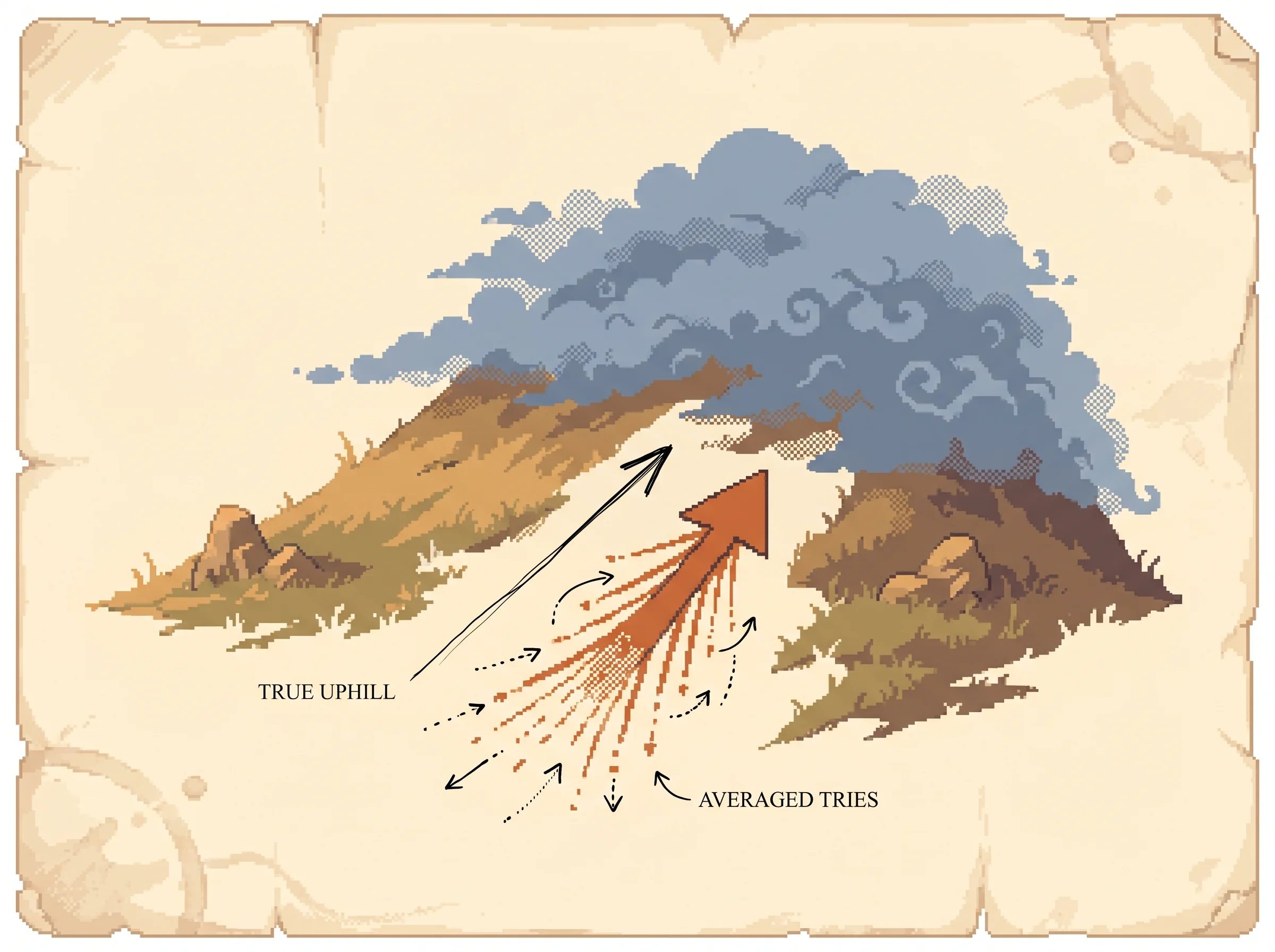
Theorem 1 makes this precise. The expected update has nonnegative inner product with the true gradient, and equals it when the learning rate is a shared constant. The simulation draws both arrows so you can watch the unit's averaged step line up with the gradient it can't compute.
The baseline. Subtracting a baseline that doesn't depend on the current output adds zero in expectation, so it never bends the direction, only shrinks the variance. Reinforcement comparison uses a running average of past reward as the baseline, which is what turns "was the reward high" into the more useful "did this try beat what I usually get."
Exploration as a learned width. A Gaussian unit outputs y from a normal distribution and learns both its mean mu and its spread sigma. The sigma update widens the search when good outcomes come from far out and narrows it when good outcomes are close to the mean, so the unit controls how much it explores on its own, separately from where.
Delayed reward. For one reward at the end of a k-step episode, accumulate each weight's eligibility across the episode and apply the update once at the end.
delta w_ij = alpha_ij (r - b_ij) sum over t of e_ij(t)Theorem 2 gives the same gradient guarantee. It needs one accumulator per weight, but it credits every step in the episode equally, which is crude and slow.
Fit with backpropagation. Put REINFORCE at the stochastic output units and backpropagation through any deterministic hidden units, and the two compose. The sum of output eligibilities is computed by an ordinary backward pass. And for a unit whose randomness is a differentiable function of its parameters, like a Gaussian written y = mu + sigma z, you can backpropagate straight through the random draw.
Results. This is an analysis paper with supporting simulations, not a benchmark. Sutton's 1984 study found that REINFORCE with reinforcement comparison outperformed the other algorithms tested on single-unit tasks. Later studies by Williams and Peng confirmed the algorithms tend to find local optima and that an entropy term in the reward helped on tasks needing structure. The Gaussian-unit experiments show sigma narrowing at a good optimum and broadening when stuck, and confirm the collapse of sigma to zero when reward stays positive and no baseline is used. There are no leaderboard numbers because there was nothing yet to benchmark against.
Limitations and open questions. There's no general convergence theory. The per-trial estimate is unbiased but high-variance, so learning is slow, and the episodic version is slower still because it spreads credit uniformly over time. Like all gradient methods it can settle on a false optimum. And the paper offers no principled way to choose the baseline that would minimize variance, which it names as the obvious next problem.
My assessment
Williams got the central thing right, and the whole field of policy gradients is the proof. The estimate he wrote down, reward above a baseline times the gradient of the log-probability of your own action, is still the exact object that PPO optimizes when it tunes a language model from human feedback. Everything between 1992 and now is stabilization bolted onto this gradient. The baseline became the value function and reward minus baseline became the advantage. A trust region and a clip stopped the policy from lurching too far in one noisy step. Minibatches and parallel rollouts beat down the variance with sheer sample count. None of that changed the gradient. It made the gradient usable.
The most impressive part is what he was honest about. He said plainly that there's no convergence guarantee, that the method is slow, that the variance is real, and that he had no principled baseline. Those four admissions are a near-complete table of contents for the next three decades of reinforcement learning research. He even wrote down the reparameterization trick, y = mu + sigma z, and the idea that a unit could learn its own exploration width, both of which the field rediscovered as load-bearing ideas much later. Naming the right problems while you solve the first version of them is rarer than solving them.
Where the work undersold itself is the framing. The title says "simple" and "connectionist," and the paper reads as a careful analysis of gradient learning for small stochastic networks, which is what it was in 1992. The slowness and variance looked then like a reason the method might stay a curiosity. What nobody could see from a Sun workstation is that this is the algorithm that scales. Pour in compute, samples, and a few variance-reduction tricks, and the same modest update trains agents to play games from pixels and aligns the largest models we build. The quiet phrase in the title, statistical gradient-following, turned out to name the workhorse of modern reinforcement learning.