Sequence to Sequence Learning with Neural Networks
One neural net reads a whole sentence into a single memory vector and a second net unrolls that vector back into the translated sentence, and reversing the input words is what made it learn.
Read at your level
Start where you're comfortable and climb as far as you like.
- For a 5-year-old
- For a high schooler
- For a college student
- For an industry pro
- For a PhD candidate
- For a peer researcher
Executive summary
Before this paper, neural networks needed inputs and outputs of a fixed size, so they couldn't turn one sentence into another. The authors fixed that with two networks. The first, the encoder, reads the source sentence one word at a time and packs the whole thing into a single fixed-length vector. The second, the decoder, reads that vector and writes the translation one word at a time until it decides to stop. On English-to-French translation the model scored 34.8 BLEU, beating a strong phrase-based system at 33.3, and reached 36.5 when used to rerank that system's guesses. The surprise was a tiny trick. Feeding the source sentence backwards jumped the score from 25.9 to 30.6, because it put the first source words next to the first target words and made the learning problem easier. The cost is the bottleneck. Cramming any sentence into one fixed vector strains on very long inputs, which the next wave of work, attention, went on to solve.
Try it
Load the Forward (long sentence fails) preset and step through it. Watch the early output words come out as UNK because their signal had to survive 9 steps and faded. Now load Reversed (long sentence works) and step again. The same words come out right, because reversing put each early source word one step from its target. Then flip the Source toggle mid-run to feel the difference live.
A 9-word sentence read in normal order. The first words sit 9 steps from their match, so their signal decays past the threshold and the decoder emits UNK for them. Watch the early outputs break.
A long sentence. Forward, the first words sit far from their matches, so the early signal decays past the threshold and the decoder emits UNK.
| source | target | lag | signal | emitted |
|---|---|---|---|---|
| the | le | 9 | 0.105 | UNK |
| small | petit | 9 | 0.105 | UNK |
| dog | chien | 9 | 0.105 | UNK |
| ran | courait | 9 | 0.105 | UNK |
| across | sur | 9 | 0.105 | UNK |
| the | le | 9 | 0.105 | UNK |
| wet | champ | 9 | 0.105 | UNK |
| green | vert | 9 | 0.105 | UNK |
| field | humide | 9 | 0.105 | UNK |
Flip a control or load a preset to start the log.
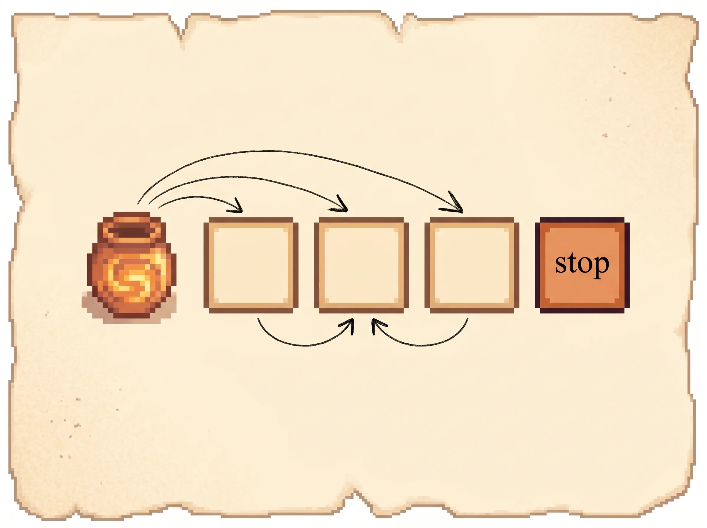
A target word comes out right only when the signal from its matching source word survives the lag between when that word entered the jar and when its translation leaves, modeled here as exp(-lag / tau). Reversing the source flips the read order, so the first source word is written last and its target follows one step later. A trained LSTM learns this carrying from data; here the decay law is fixed so the pattern is legible. The recovery threshold is fixed at 0.12 — a signal must reach at least this level to count as recovered. This runs sentences of up to 9words; the paper's LSTM ran 4 layers of 1000 cells over sentences of any length.
For a 5-year-old
Imagine a friend who has to carry a message across a long hallway. You whisper a word to them at one end. They walk all the way to the other end and try to say it back. If the hallway is short, they remember the word fine. If the hallway is really long, they forget the start by the time they get there.
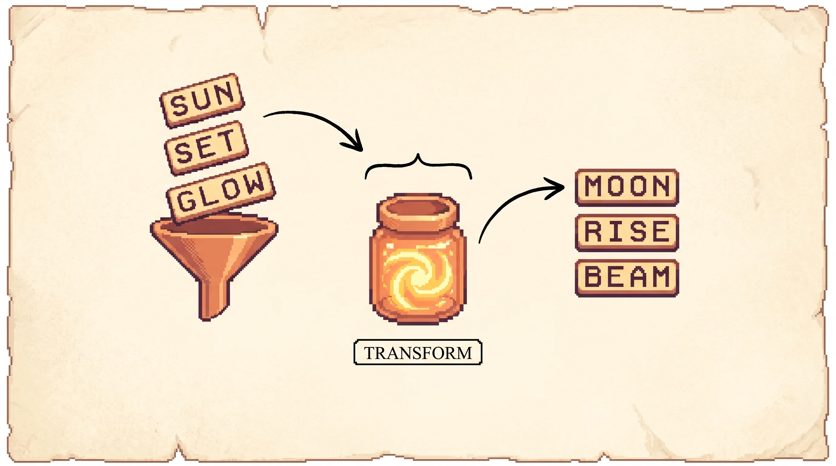
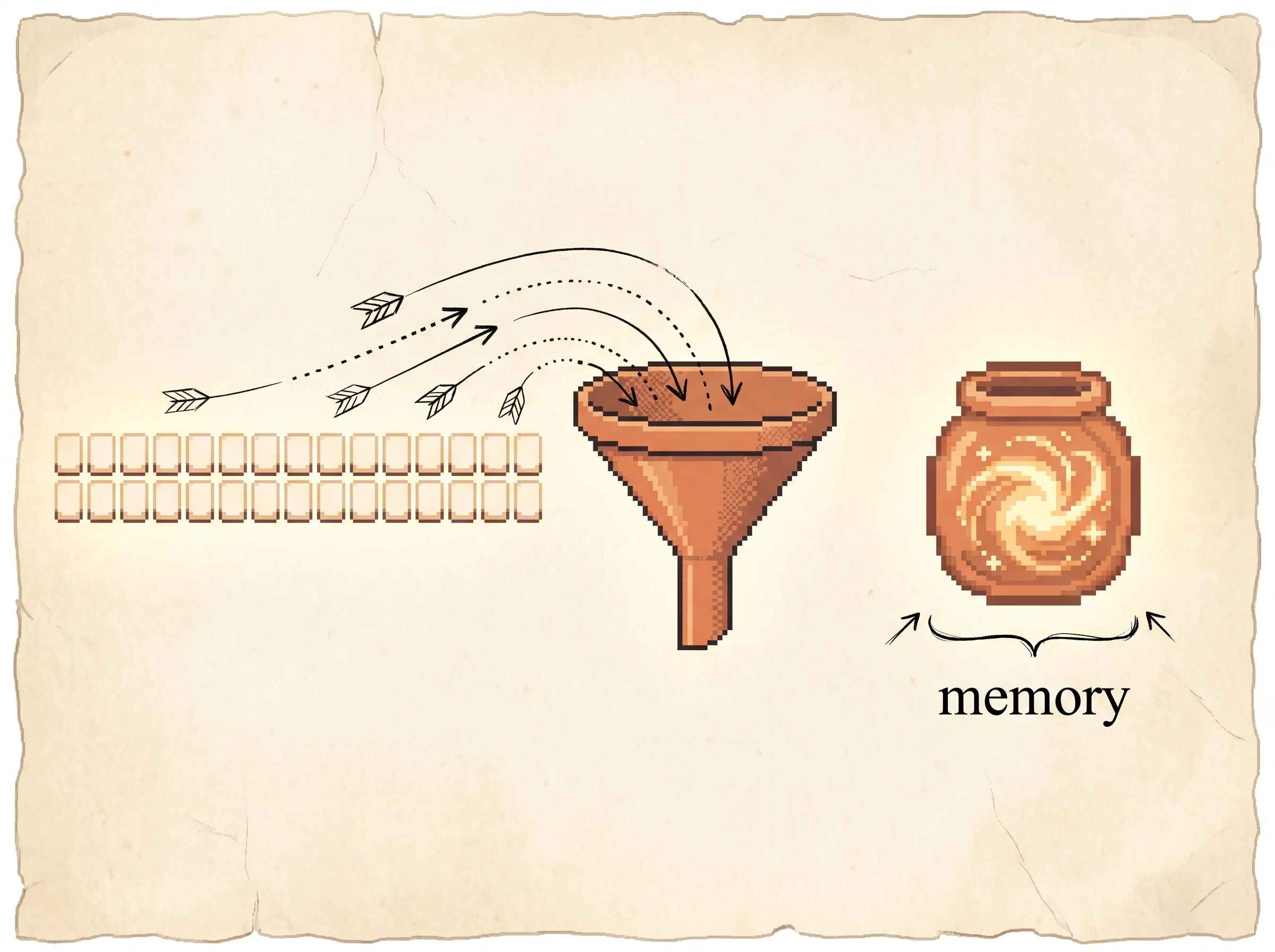
A computer that translates works like two of these friends. The first friend listens to a whole sentence, word by word, and squeezes it all into one little jar of memory. The second friend takes the jar and says the sentence back in a new language, one word at a time, until it reaches the end and stops.
Here's the funny part. The first word you whisper has the longest hallway to walk, so it gets forgotten the most. Somebody figured out a trick. Say the sentence backwards to the first friend. Now the word that needs to come out first only has a tiny hallway to walk, so it stays fresh. Nothing about the words changed. Only the order they walked in. And it worked way better.
Real computers don't whisper or walk. The memory is a list of numbers, and the forgetting is the numbers fading as they pass through many steps. But the feeling is the same. A short trip means a clear memory.
For a high schooler
Your phone's keyboard guesses your next word from the words before it. That works because it reads left to right and keeps a little running memory. But a translator has a harder job. The English sentence and the French sentence aren't the same length, and the words don't line up one for one. You can't just guess the next word, you have to read the whole thing first.
The fix uses two networks. Here's the one term for this section. An encoder is a network that reads the input sentence word by word and updates a memory as it goes, so after the last word the memory holds a summary of everything. The decoder is a second network that starts from that summary and produces the output sentence, one word at a time, feeding each word it writes back in to help pick the next one. It keeps going until it writes a special stop word.
Here's the catch with a worked example. Say you feed in "the dog ran" and the memory has to carry "the" all the way through reading "dog" and "ran" before the decoder even starts. That's a long carry for the first word. Now feed it backwards as "ran dog the". The word "the" goes in last, so when the decoder asks for it first, the memory is still fresh. The total carrying distance across all the words stays the same. But the first few words got way easier, and those early wins make the whole thing train better.
A short carry means a clear memory, which is why the order you feed the words in matters.
For a college student
You should care because this is the paper that showed a plain neural network could beat a hand-engineered translation system end to end, with almost no assumptions baked in. The motivation was a hard limit of deep nets. They map fixed-size vectors to fixed-size vectors, so a sentence of unknown length had no clean way in. Recurrent nets handle variable length, but a standard RNN struggles to carry information across many steps because the gradient that has to flow back across that distance vanishes.
The idea is to use a Long Short-Term Memory network, an RNN built to hold information across long gaps, as both halves. The encoder LSTM reads the input (x_1, ..., x_T) and its final hidden state becomes a fixed vector v. The decoder LSTM models the probability of the output sequence conditioned on v.
p(y_1, ..., y_T' | x_1, ..., x_T) = product over t of p(y_t | v, y_1, ..., y_{t-1})Read it left to right. The whole input collapses into v. Then each output word y_t is predicted from v and every output word so far, using a softmax over the vocabulary. Each sentence ends with an end-of-sequence token, so the model can handle outputs of any length and knows when to stop.
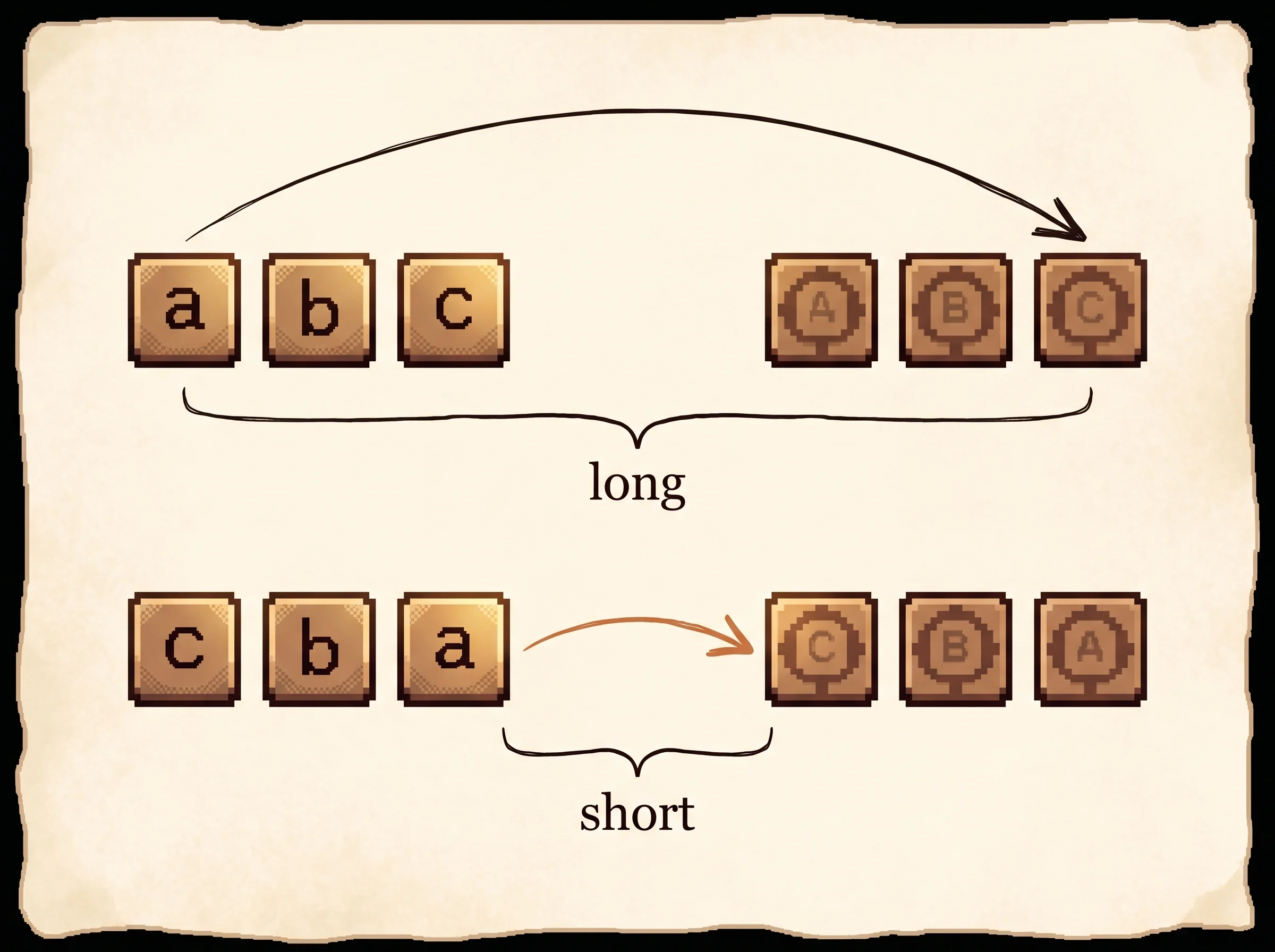
The bottleneck is the whole game. However long the source sentence, it has to fit into one v. The reason this trains at all on long inputs is the reversal trick, and it pays off because of the gradient path. Map a, b, c to α, β, γ. Read forward, the source word a sits 3 steps from α, so the signal connecting them is weak. Read backward as c, b, a, and a sits right next to α. The average distance between matched words doesn't change, but the minimum distance for the early words drops to near zero, and those short-range links give the optimizer something easy to grab onto first.
The simulation above makes this exact effect concrete. The lag column is the number of steps each word's signal had to survive, and signal is what's left of it. Reverse the source and watch the first word's lag fall from the sentence length to 1.
The limitation falls straight out of the single v. The vector is fixed size, so very long sentences get compressed harder, and quality eventually suffers. The model here did fine up to about 35 words, but the squeeze is real.
For an industry pro
The problem it solves is mapping one variable-length sequence to another without hand-building an alignment, which is exactly machine translation, summarization, speech-to-text, and question answering. Before this, you wired up a phrase table and a language model and a reordering model by hand. This replaces all of it with one trained net.
Deployment cost in this paper was steep for the era. A 4-layer LSTM with 1000 cells per layer, 384M parameters, trained for about 10 days on 8 GPUs, one layer per GPU. Inference is sequential on the decoder side, one token at a time, so latency scales with output length. The single fixed vector means memory cost per example is bounded regardless of input length, which is cheap, but it's also the thing that caps quality on long inputs.
The improvement over the standard at the time was real. A pure neural system hit 34.8 BLEU against a phrase-based baseline at 33.3, the first time a neural translator beat a strong phrase-based system on a large task, and reranking that system's 1000-best list pushed it to 36.5. The failure mode to plan around is the bottleneck plus the limited vocabulary. The model used a fixed 80,000-word output vocabulary and emitted a generic UNK token for anything outside it, so rare names and numbers came out wrong. If your domain has lots of rare tokens, budget for that. And reverse your inputs. It's a free preprocessing step that bought 4 to 5 BLEU here.
For a PhD candidate
The contribution is showing that a general, assumption-light encoder-decoder LSTM does direct sequence transduction at a level that beats a tuned phrase-based SMT system on WMT'14 English-to-French. Kalchbrenner and Blunsom first mapped a sentence to a vector and back, but with a convolutional encoder that loses word order. Cho et al. used an LSTM-like encoder-decoder but only to rescore an SMT system rather than translate directly. This paper translates directly and wins.
The methodological choices reward scrutiny. Using two separate LSTMs, one to encode and one to decode, costs almost nothing and leaves room to train on multiple language pairs. Going deep, 4 layers, cut perplexity by nearly 10 percent per added layer over shallow LSTMs, which is the kind of depth-helps result that motivated later scaling. The reversal trick is the headline empirical finding. It dropped test perplexity from 5.8 to 4.7 and raised BLEU from 25.9 to 30.6, and the authors' explanation is the reduction in minimal time lag between corresponding source and target positions, which eases the credit-assignment problem early in the output. They also enforced a hard gradient-norm constraint, which mattered because LSTMs avoid vanishing gradients but can still explode.
Threats to validity worth probing. The reversal explanation is plausible and the gain is large, but it rests on intuition about short-term dependencies rather than a controlled measurement of where the gradient flows. The single fixed-length v is an obvious information bottleneck, yet the model held up to about 35 words, which the authors found surprising and which suggests the LSTM uses the vector cleverly rather than as a simple average. The PCA plots show representations sensitive to word order and invariant to active-versus-passive voice, which is suggestive of meaningful structure but is a handful of examples, not a systematic probe. The open question this paper hands forward is the bottleneck itself, and Bahdanau-style attention, which the authors cite, is exactly the answer the field reached for next.
For a peer researcher
The delta against Cho et al. is that this model translates directly and competitively instead of only rescoring, and the delta against Kalchbrenner and Blunsom is keeping word order by using a recurrent encoder rather than a convolutional one. Strip it down and the model is two deep LSTMs and a softmax, trained to maximize log p(T | S), decoded with a small beam where even beam size 2 captures most of the gain.
The choices read as deliberate tradeoffs. The fixed vector v trades the ability to look back at the source for a clean, bounded interface between encoder and decoder, and the reversal trick is a cheap patch on the cost of that choice rather than a fix for it. Reversing trades nothing measurable, the average token distance is unchanged, for a large gain in early-output trainability, which tells you the optimization landscape, not the representational capacity, was the binding constraint at this scale. Depth over width was the other bet, and it paid.
What would change my mind on the framing. If a model without the single-vector bottleneck matched this at the same compute, the encode-to-one-vector story would look like a detour rather than a milestone, and that's close to what happened. Attention removed the bottleneck within a year and the reversal trick became unnecessary, because once the decoder can attend to any source position the minimal-time-lag problem dissolves. The lasting contribution isn't the architecture, it's the demonstration that end-to-end neural transduction beats a hand-built pipeline, which set the direction for everything after.
How it works
The problem and why prior approaches failed. Deep neural networks need fixed-dimensional inputs and outputs, so they can't map a sentence of one length to a sentence of another. Recurrent networks handle variable length by reading one token at a time and carrying a hidden state, but a plain RNN can't learn long-range dependencies, because the signal connecting a far-apart input and output has to survive many steps and the gradient through them vanishes. Convolutional encoders parallelize but throw away word order.
The key idea. Use an LSTM, which is built to carry information across long gaps, as an encoder that reads the whole source into one fixed vector v, then a second LSTM as a decoder that generates the target from v one token at a time.
Methodology. Two deep LSTMs, 4 layers each, 1000 cells and 1000-dimensional embeddings per layer, a 160,000-word input vocabulary and an 80,000-word output vocabulary, 384M parameters total. The training objective maximizes the log probability of the correct translation T given the source S over the training set S.
maximize (1 / |S|) sum over (T, S) in S of log p(T | S)At test time the model outputs the most likely translation under a left-to-right beam search.
T_hat = argmax over T of p(T | S)The beam keeps the B best partial hypotheses, extends each by every possible next word, and prunes back to B. A hypothesis leaves the beam when it emits the end-of-sequence token. The decoder works well even at beam size 1, and beam size 2 captures most of the benefit.
Three details made it train. They used two separate LSTMs so the encoder and decoder don't share parameters. They went deep, since each extra layer cut perplexity by nearly 10 percent. And they reversed the source sentence, the single most important trick.
forward:   map  a b c   to   α β γ      (a is 3 steps from α)
reversed:  map  c b a   to   α β γ      (a is 1 step from α)
Reversing leaves the average distance between matched words unchanged but slashes the minimal distance for the first few, which introduces many short-term dependencies and makes optimization much easier. In the simulation, the per-word lag column shows this directly. Load the long sentence forward and the first word's lag equals the sentence length. Flip to reversed and it drops to 1.
Results with effect sizes. Reversing the source cut test perplexity from 5.8 to 4.7 and raised BLEU from 25.9 to 30.6. An ensemble of 5 reversed LSTMs with beam size 12 scored 34.81 BLEU on WMT'14 English-to-French, against a phrase-based baseline at 33.30, the first pure neural system to beat a strong phrase-based system on a large task. Using the LSTM to rerank the baseline's 1000-best list reached 36.5, within 0.5 BLEU of the best published result. Quality held steady on sentences up to about 35 words with only minor degradation on the longest.
Limitations and open questions. The fixed-length vector is a hard bottleneck, so very long sentences get compressed too aggressively. The 80,000-word output vocabulary forces a generic UNK token for rare words, which penalized the BLEU score. And the reversal explanation, while backed by a large measured gain, rests on an intuition about short-term dependencies rather than a direct measurement. The cited fix, an attention mechanism that lets the decoder look back at the source, is where the field went next.
My assessment
The authors got the big call right. End-to-end neural transduction works, and it can beat a hand-built pipeline, which was not obvious in 2014 and reset the whole direction of the field. The cheapest idea in the paper turned out to be the most memorable. Reversing the input is a one-line preprocessing change that bought 4 to 5 BLEU, and the honesty about why, short-term dependencies easing optimization rather than some deep representational gain, is the right read. It says the bottleneck back then was the optimization landscape, not the model's capacity, and that lesson generalized.
Where the paper was constrained is the same place it pointed. The single fixed vector is a beautiful clean interface and a real ceiling, and the reversal trick is a patch on that ceiling, not a removal of it. The authors saw this, cited the attention work that would dissolve the problem, and within a year reversal became a historical footnote because attention let the decoder reach any source position directly. The fixed vocabulary and the UNK problem were the other soft spot, since a translator that mangles names and numbers has a real production limit. None of that dents the core. This is the paper that made sequence-to-sequence a default tool, and the encoder-decoder framing it established still shapes how the field thinks about turning one sequence into another.